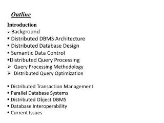
Introduction Background Distributed DBMS Architecture Distributed Database Design
Outline. Introduction Background Distributed DBMS Architecture Distributed Database Design Semantic Data Control Distributed Query Processing Query Processing Methodology Distributed Query Optimization Distributed Transaction Management Parallel Database Systems

Introduction Background Distributed DBMS Architecture Distributed Database Design
E N D
Presentation Transcript
Outline • Introduction • Background • Distributed DBMS Architecture • Distributed Database Design • Semantic Data Control • Distributed Query Processing • Query Processing Methodology • Distributed Query Optimization • Distributed Transaction Management • Parallel Database Systems • Distributed Object DBMS • Database Interoperability • Current Issues
Query Processing high level user query low level data manipulation commands
Query Processing Components Query language that is used ➠ SQL: “intergalactic data speak” Query execution methodology ➠ The steps that one goes through in executing high-level (declarative) user queries. Query optimization ➠ How do we determine the “best” execution plan?
Selecting Alternatives SELECT ENAME FROM EMP,ASG WHERE EMP.ENO = ASG.ENO AND DUR > 37 Strategy 1 ΠENAME(σDUR>37∧EMP.ENO=ASG.ENO=(EMP × ASG)) Strategy 2 ΠENAME(EMP ENO (σDUR>37(ASG))) Strategy 2 avoids Cartesian product, so is “better”
What is the Problem? Site 1: Site 2: ASG2=σENO>“E3”(ASG) ASG1=σENO≤“E3”(ASG) Site 3: Site 4: EMP1=σENO≤“E3”(EMP) EMP2=σENO>“E3”(EMP) Site 5: Result
Site 5 Site 5 EMP1 EMP2 ASG1 ASG2 EMP1 EMP2 Site 1 Site 2 Site 3 Site 4 Site 3 Site 4 ASG1 ASG2 Site 1 Site 2
Cost of Alternatives Assume: size(EMP) = 400, size(ASG) = 1000 tuple access cost = 1 unit; tuple transfer cost = 10 units • Strategy 1 • . produce ASG': (10+10)∗tuple access cost 20 • 2.transfer ASG' to the sites of EMP: (10+10)∗tuple transfer cost 200 • 3.produce EMP': (10+10) ∗tuple access cost∗ 240 • 4. transfer EMP' to result site: (10+10) ∗tuple transfer cost 200 • Total cost 460 Strategy 2 1.transfer EMP to site 5:400∗tuple transfer cost 4,000 2.transfer ASG to site 5 :1000∗tuple transfer cost 10,000 3.produce ASG':1000∗tuple access cost 1,000 4. join EMP and ASG':400∗20∗tuple access cost 8,000 Total cost 23,000
Query Optimization Objectives Minimize a cost function I/O cost + CPU cost + communication cost These might have different weights in different distributed environments Wide area networks ➠ communication cost will dominate low bandwidth low speed high protocol overhead ➠ most algorithms ignore all other cost components Local area networks ➠ communication cost not that dominant ➠ total cost function should be considered Can also maximize throughput
Complexity of Relational Operations Assume ➠ relations of cardinality n ➠ sequential scan
Query Optimization Issues – Types of Optimizers Exhaustive search ➠ cost-based ➠ optimal ➠ combinatorial complexity in the number of relations Heuristics ➠ not optimal ➠ regroup common sub-expressions ➠ perform selection, projection first ➠ replace a join by a series of semijoins ➠ reorder operations to reduce intermediate relation size ➠ optimize individual operations
Query Optimization Issues – Optimization Granularity Single query at a time ➠ cannot use common intermediate results Multiple queries at a time ➠ efficient if many similar queries ➠ decision space is much larger
Query Optimization Issues – Optimization Timing Static ➠ compilation optimize prior to the execution ➠ difficult to estimate the size of the intermediate results error propagation ➠ can amortize over many executions ➠ R* Dynamic ➠ run time optimization ➠ exact information on the intermediate relation sizes ➠ have to reoptimize for multiple executions ➠ Distributed INGRES Hybrid ➠ compile using a static algorithm ➠ if the error in estimate sizes > threshold, reoptimize at run time ➠ MERMAID
Query Optimization Issues – Statistics Relation ➠ cardinality ➠ size of a tuple ➠ fraction of tuples participating in a join with another relation Attribute ➠ cardinality of domain ➠ actual number of distinct values Common assumptions ➠ independence between different attribute values ➠ uniform distribution of attribute values within their domain
Query Optimization Issues –Decision Sites Centralized ➠ single site determines the “best” schedule ➠ simple ➠ need knowledge about the entire distributed database Distributed ➠ cooperation among sites to determine the schedule ➠ need only local information ➠ cost of cooperation Hybrid ➠ one site determines the global schedule ➠ each site optimizes the local subqueries
Query Optimization Issues –Network Topology Wide area networks (WAN) – point-to-point ➠ characteristics low bandwidth low speed high protocol overhead ➠ communication cost will dominate; ignore all other cost factors ➠ global schedule to minimize communication cost ➠ local schedules according to centralized query optimization Local area networks (LAN) ➠ communication cost not that dominant ➠ total cost function should be considered ➠ broadcasting can be exploited (joins) ➠ special algorithms exist for star networks
Step 1 – Query Decomposition Input : Calculus query on global relations Normalization ➠ manipulatequeryquantifiers and qualification Analysis ➠ detect and reject “incorrect” queries ➠ possible for only a subset of relational calculus Simplification ➠ eliminate redundant predicates Restructuring ➠ calculus query Τalgebraic query ➠ more than one translation is possible ➠ use transformation rules
Normalization Lexical and syntactic analysis ➠ check validity (similar to compilers) ➠ check for attributes and relations ➠ type checking on the qualification Put into normal form ➠ Conjunctive normal form (p11∨p12∨…∨p1n) ∧…∧ (pm1∨pm2∨…∨pmn) ➠ Disjunctive normal form (p11∧p12 ∧…∧p1n) ∨…∨ (pm1 ∧pm2∧…∧Τpmn) ➠ OR's mapped into union ➠ AND's mapped into join or selection
Analysis Refute incorrect queries Type incorrect ➠ If any of its attribute or relation names are not defined in the global schema ➠ If operations are applied to attributes of the wrong type Semantically incorrect ➠ Components do not contribute in any way to the generation of the result ➠ Only a subset of relational calculus queries can be tested for correctness ➠ Those that do not contain disjunction and negation ➠ To detect: connection graph (query graph) join graph
Analysis – Example SELECT ENAME,RESP FROM EMP, ASG, PROJ WHERE EMP.ENO = ASG.ENO AND ASG.PNO = PROJ.PNO AND PNAME = "CAD/CAM" AND DUR ≥ 36 AND TITLE = "Programmer"
Analysis If the query graph is not connected, the query is wrong. SELECT ENAME,RESP FROM EMP, ASG, PROJ WHERE EMP.ENO = ASG.ENO AND PNAME = "CAD/CAM" AND DUR ≥ 36 AND TITLE = "Programmer"
Simplification Why simplify? ➠ Remember the example How? Use transformation rules ➠ elimination of redundancy idempotency rules p1 ∧ ¬( p1) ⇔ false p1 ∧ (p1 ∨ p2) ⇔ p1 p1 ∨ false ⇔ p1 … ➠ application of transitivity ➠ use of integrity rules
Simplification – Example SELECT TITLE FROM EMP WHERE EMP.ENAME = “J. Doe” OR (NOT(EMP.TITLE = “Programmer”) AND (EMP.TITLE = “Programmer” OR EMP.TITLE = “Elect. Eng.”) AND NOT(EMP.TITLE = “Elect. Eng.”)) SELECT TITLE FROM EMP WHERE EMP.ENAME = “J. Doe”
Restructuring • Convert relational calculus to • relational algebra • Make use of query trees • Example • Find the names of employees other than • J. Doe who worked on the CAD/CAM • project for either 1 or 2 years. • SELECT ENAME • FROM EMP, ASG, PROJ • WHERE EMP.ENO = ASG.ENO • AND ASG.PNO = PROJ.PNO • AND ENAME ≠ “J. Doe” • AND PNAME = “CAD/CAM” • AND (DUR = 12 OR DUR = 24)
Restructuring – Transformation Rules • Commutativity of binary operations • ➠ R × S ⇔ S × R • ➠ R S ⇔S R • ➠ R ∪ S ⇔ S ∪ R • Associativity of binary operations • ➠ ( R × S ) × T ⇔ R × (S × T) • ➠ ( R S) T ⇔ R (S T) • Idempotence of unary operations • ➠ ΠA’(ΠA’(R)) ⇔ΤΠA’(R) • ➠ σp1(A1)(σp2(A2)(R)) = σp1(A1) ∧ p2(A2)(R) • where R[A] and A' ⊆ A, A" ⊆ A and A' ⊆ A" • Commuting selection with projection
Restructuring – Transformation Rules • Commuting selection with binary operations • ➠ σp(A)(R × S) ⇔ (σp(A) (R)) × S • ➠ σp(Ai)(R (Aj,Bk) S) ⇔ (σp(Ai) (R)) (Aj,Bk) S • ➠ σp(Ai)(R ∪ T) ⇔ σp(Ai) (R) ∪ σp(Ai) (T) • where Ai belongs to R and T • Commuting projection with binary operations • ➠ ΠC(R × S) ⇔ΠA’(R) × ΠΤB’(S) • ➠ ΠC(R (Aj,Bk) S) ⇔ΠA’(R) (Aj,Bk) ΠB’(S) • ➠ ΠC(R ∪ S) ⇔ΠC (R) ∪ ΠC (S) • where R[A] and S[B]; C = A' ∪ B' where A' ⊆ A, B' ⊆ B
Example Recall the previous example: Find the names of employees other than J. Doe who worked on the CAD/CAM project for either one or two years. SELECT ENAME FROM PROJ, ASG, EMP WHERE ASG.ENO=EMP.ENO AND ASG.PNO=PROJ.PNO AND ENAME≠“J. Doe” AND PROJ.PNAME=“CAD/CAM” AND (DUR=12 OR DUR=24)
Step 2 – Data Localization • Input: Algebraic query on distributed relations • Determine which fragments are involved • Localization program • ➠ substitute for each global query its materialization • program • ➠ optimize
Example Assume ➠ EMP is fragmented into EMP1, EMP2, EMP3 as follows: EMP1=σENO≤“E3”(EMP) EMP2= σ“E3”<ENO≤“E6”(EMP) EMP3=σENO≥“E6”(EMP) ➠ ASG fragmented into ASG1 and ASG2 as follows: ASG1=σENO≤“E3”(ASG) ASG2=σENO>“E3”(ASG) Replace EMP by (EMP1∪EMP2∪EMP3 ) and ASG by (ASG1 ∪ ASG2) in any query
Step 3 – Global Query Optimization Input: Fragment query Find the best (not necessarily optimal) global schedule ➠ Minimize a cost function ➠ Distributed join processing Bushy vs. linear trees Which relation to ship where? Ship-whole vs ship-as-needed ➠ Decide on the use of semijoins Semijoin saves on communication at the expense of more local processing. ➠ Join methods nested loop vs ordered joins (merge join or hash join)
Cost-Based Optimization • Solution space • ➠ The set of equivalent algebra expressions (query trees). • Cost function (in terms of time) • ➠ I/O cost + CPU cost + communication cost • ➠ These might have different weights in different distributed • environments (LAN vs WAN). • ➠ Can also maximize throughput • Search algorithm • ➠ How do we move inside the solution space? • ➠ Exhaustive search, heuristic algorithms (iterative • improvement, simulated annealing, genetic,…)
Search Space • Search space characterized by • alternative execution plans • Focus on join trees • For N relations, there are O(N!) • equivalent join trees that can be • obtained by applying • commutativity and associativity • rules • SELECT ENAME,RESP • FROM EMP, ASG, PROJ • WHERE EMP.ENO=ASG.ENO • AND ASG.PNO=PROJ.PNO
Search Space • Restrict by means of heuristics • ➠ Perform unary operations before binary operations • Restrict the shape of the join tree • ➠ Consider only linear trees, ignore bushy ones Linear Join Tree Bushy Join Tree
Search Strategy • How to “move” in the search space. • Deterministic • ➠ Start from base relations and build plans by adding one • relation at each step • ➠ Dynamic programming: breadth-first • ➠ Greedy: depth-first • Randomized • ➠ Search for optimalities around a particular starting point • ➠ Trade optimization time for execution time • ➠ Better when > 5-6 relations • ➠ Iterative improvement
Search Strategies • Deterministic • Randomized
Cost Functions • Total Time (or Total Cost) • ➠ Reduce each cost (in terms of time) component • individually • ➠ Do as little of each cost component as possible • ➠ Optimizes the utilization of the resources • Increases system throughput • Response Time • ➠ Do as many things as possible in parallel • ➠ May increase total time because of increased total activity
Total Cost Summation of all cost factors Total cost = CPU cost + I/O cost + communication cost CPU cost = unit instruction cost ∗ no.of instructions I/O cost = unit disk I/O cost ∗ no. of disk I/Os communication cost = message initiation + transmission
Total Cost Factors • Wide area network • ➠ message initiation and transmission costs high • ➠ local processing cost is low (fast mainframes or minicomputers) • ➠ ratio of communication to I/O costs = 20:1 • Local area networks • ➠ communication and local processing costs are more • or less equal • ➠ ratio = 1:1.6
Response Time Elapsed time between the initiation and the completion of a query Response time = CPU time + I/O time + communication time CPU time = unit instruction time∗no. of sequential instruction I/O time = unit I/O time ∗ no. of sequential I/Os communication time = unit msg initiation time ∗ no. of sequential msg + unit transmission time ∗ no. of sequential bytes
Example Assume that only the communication cost is considered Total time = 2 ∗ message initialization time + unit transmission time ∗ (x+y) Response time = max {time to send x from 1 to 3, time to send y from 2 to 3} time to send x from 1 to 3 = message initialization time + unit transmission time ∗ x time to send y from 2 to 3 = message initialization time + unit transmission time ∗ y
Optimization Statistics • Primary cost factor: size of intermediate relations • Make them precise more costly to maintain • ➠ For each relation R[A1, A2, …, An] fragmented as R1, …, Rr • length of each attribute: length(Ai) • the number of distinct values for each attribute in each fragment: card(ΠAiRj) • maximum and minimum values in the domain of each attribute: • min(Ai), max(Ai) • the cardinalities of each domain: card(dom[Ai]) • the cardinalities of each fragment: card(Rj) • ➠ Selectivity factor of each operation for relations • For joins
Intermediate Relation Sizes Selection where
Intermediate Relation Sizes Projection card(ΠA(R))=card(R) Cartesian Product card(R × S) = card(R) ∗card(S) Union upper bound: card(R ∪ S) = card(R) + card(S) lower bound: card(R ∪ S) = max{card(R), card(S)} Set Difference upper bound: card(R–S) = card(R) lower bound: 0
Intermediate Relation Sizes Join ➠ Special case: A is a key of R and B is a foreign key of S; ➠ More general: Semijoin where
Centralized Query Optimization • INGRES • ➠ dynamic • ➠ interpretive • System R • ➠ static • ➠ exhaustive search