Introduction to Linear Classifiers: Linear Discriminant Functions
Learn about linear classifiers, focusing on linear discriminant functions for optimal decision-making. Understand their construction, properties, and training methods for practical applications. Explore different approaches and algorithms like the perceptron learning rule.

Introduction to Linear Classifiers: Linear Discriminant Functions
E N D
Presentation Transcript
Introduction • Remember that Bayes’ decision rule requires the knowledge of eitherP(Ci|X) or P(X|Ci) and P(Ci) • We showed how to create an estimate for P(X|Ci) using one Gaussian curve or a mixture of Gaussians • We also showed that modeling the distributions implicitly models the discriminant functions as well • However, in practice we will always have a mismatch between the assumed and the real shape of the distribution • Also, for the classification we don’t need the distributions,just the discriminant functions • This gives the idea to model the discriminant functionsdirectly • Seems to be an easier problem than estimating distributions
Some naming conventions • Decision surface models • Also called “discriminative models” (they focus on discriminating the classes) • More related to the estimation of P(Ci|X) • Earlier I called this the “geometric approach” • They model the geometry of the decision surface • Class distribution models • Also called “generative models” (they can be used to generate samples from a class) • More related to the estimation of P(X|Ci) • Earlier I called this the “decision theoretic approach” • They require a decision mechanism for classification • However, the two classes are not perfectly disjunct, e.g. there are discriminative training methods for GMMs (they optimize the estimate for P(Ci|X) instead of P(X|Ci)…)
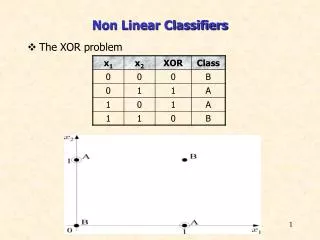
Linear classifiers • Today we focus on methods that directly model the discriminant functions • As the simplest case, we will study the case of linear discriminant functions • We know that they are optimal in the case of Gaussian class distributions with equal covariances • They may not be optimal for other distributions, but they are very easy to use • While they will perform poor for most practical problems, they will form the basis of two of the best machine learning approaches, neural networks and support vector machines • First, we will discuss the case of having only 2 classes • Later we will see how to extend the methods to more classes
Linear discriminant functions • A discriminant function is called linear if it has the form • Where w is the weight vector and w0 is the bias or threshold • The linear discriminant function is a line in 1D, plane in 2D,… • The decision boundary is where • It is a point in 1D, a line in 2D, a plane in 3D, …
Some coordinate geometry… • w determines the orientation of the decision hyperplane • It is the normal vector of the plane • w0 determines the location of thedecision hyperplane • Note that multiplying g(x) by a constantchanges the steepness of the discriminant function, but won’t change the decision surface • So the distance of a point x from the decision surface is given by
Simplifying the notation • We simplify the notation by fusing w0 into w • Instead of (w1, w2, … wd) we use the weight vector a=(w0, w1, w2, …wd) • And we also augment the feature vector as: y=(1, x1, x2,…,xd) • With this, instead of we can write • So we have a homogeneousdiscriminant function • The decision boundary goes through the origin
Training the linear classifier • Given samples from c1 and c2, how can we select the weight so that the classification error is zero? • Remember that • So the classification error is zero if • Equivalently, the error is zero if • We prefer this form, so we multiply all samples from c2 by -1 • We call this step the “problem normalization step” • Now we can formalize the goal of training as finding a weight vector afor which
Visualizing the classification problem • All vectors from the shaded region give a good solution • So usually there is no unique solution, rather a solution region We seek a hyperplane that separates the samples We seek a hyperplane that puts the normalized samples on the same side
Training the linear classifier • The goal of training is to find a weight vector a for which • We will examine several methods for this • The perceptron algorithm will give an iterative solution • The linear regression method will define an error functionand solve thins by a closed-form solution • The gradient descent method optimizes the same error function by an iterative solution • Then we modify the error function, which leads to the Ho-Kayshap procedure • Or we can generalize the linear discriminant function, which leads to logistic regression • This also creates a solution which is related to Bayes’ decision theory!
The perceptron learning rule • Rosenblatt invented the linear classifier as the “perceptron” in 1957 • He also proposed a training method that was called the perceptron learning rule • He pointed out the similarity of the model to biological neurons • This was the origin of the “artificial neural network” research field • The perceptron learning rule • It is an iterative algorithm (goes through the training samples many times) • If a sample is correctly classified, it does nothing • If a sample is misclassified, it modifies the weights • If the 2 classes are linearly separable, then it finds a good solution in finite steps • However, it guarantees nothing when there is no solution • This is why we will prefer other methods later
The perceptron learning rule • Proof that it modifies the weights in the good direction: • Remember that a sample is misclassified if • In that case, the algorithm updates a: • Then the output value changes as:
Variants of the perceptron learning rule • The perceptron update rule modifies the weights after each sample • This is what we call on-line learning • The off-line of batch variant updates the weights using all misclassified samples: • Where Yk is the set of all misclassified samples • η(k) is the learning rate (a small positive value, which is constant or gradually decreases as the iteration count k increases)
Visualization • Red curve: decision surface before iteration (y is on the wrong side) • Green curve: decision surface after iteration (y is on the proper side)
Training by optimizing a target function • This group of methods requires us to quantify the error of the classifier by some function • This function is called the error function, cost function, objective function, target function,… • The parameters of this function will be the weights • We will find a proper set of parameters by optimizing the target function • This turns the machine learning problem into an optimization problem • In the simplest case we can find the global optimum by a closed formula • In more complex cases we will use iterative algorithms • In the most complex cases these iterative algorithms will guarantee only to find a local optimum, not a global optimum
The gradient descent optimization algorithm • The simplest general optimization algorithm for multivariate functions • Suppose that we want to minimize a function of many variables • We know that in the minimum point the derivative is zero • So, theoretically, we should calculate the partial derivatives and set them to zero • However, in many practical cases we cannot solve this analytically • The gradient descent algorithm iteratively decreases the target function by stepping in the direction of the steepest decrease, which direction is given by the gradient vector
The weaknesses of gradient descent • Gradient descent may stuck in a local optimum • If the learning rate is too small, the algorithm converges too slowly • If the learning rate is too large, we won’t find the optimum • We usually start with a large learning rate and gradually decrease it
Variants of gradient descent • We usually define the error of the actual model (actual parameter set) as the sum of value of the error function over all samples • In this case, the gradient descent algorithm is very similar to the off-line or batch version of the perceptron algorithm • However, we can also apply the on-line or semi-batch version of the algorithm – we process the training data in batches • In this case we calculate the error only over one sample or a subset (batch) of the samples before updating the weights • This version is known as stochastic gradient descent (SGD): • By calculating the error over a different subset of the samples in each iteration, weoptimize a slightly different version of the original target function (which is defined as the error over all samples) • This introduces a slight randomness into the process • In practice it is not harmful, but in fact helps avoid local optima, and also makes convergence faster
The mean squared error (MSE) • We want to find a weight vector a for which • Let’s define a target value bi for each sample, so that • And define the error of the training as • This is the mean squared error function • And the problem is turned into a regression task • In this case it is a linear task, also known as least squares linear regression • What are good target values for bi? • The should be positive • In lack of further information, we can use
Least squares linear regression • We need to solve n linear equations • In matrix notation: • So, shortly, we have to solve
Least squares linear regression • We need to solve a linear systemwhere the size of the Y matrix is n times d+1(n is the number of examples, d is the number of features) • If n=d+1, then Y is a square matrix, and if Y is nonsingular, then there is exactly one solution: • But this rarely happens in practice • Usually the number of examples is much higher than the number of features • In this case the equation system is overdetermined (we have more equations that unknowns), so there is no exact solution • That is, the MSE error cannot be 0 • But we can still find a solution that minimizes the MSE error function
Minimizing the MSE error • We minimize the MSE error by calculating its gradient • Then we set the gradient to zero • If the inverse of YtY exists, there is a unique solution • (YtY)-1Yt is called the Moore-Penrose pseudo-inverse of Y, because
Minimizing the MSE error using gradient descent • We can also use the gradient descent optimization procedure to find the minimum of the MSE error function • In this case, it is also guaranteed to find the global optimum, because the error surface is a quadratic bowl, it has no local optima(we have to take care to gradually decrease the learning rate, though) • Why would we prefer an iterative solution when there is a closed form solution? • In n or/and d is large, working with the Y matrix may be too costly (matrix multiplication/inversion) • If Y is close to singular (e.g. some samples are highly correlated) the matrix inversion may become numerically instable
Problems with the least squares linear regression approach • We set the target value to 1 for all positive examples, and to -1 for all negative examples (remember the normalization step!) • This is what we are trying to do in 1D: • This is what happens when a sample is too far in the good side:
Problems with linear regression • Another example in 2D (showing only the decision surface): • The algorithm pays too much attention to samples that are far away from the decision surface • Some possible solutions • Modify the target values Ho-kashyap procedure • Modify (generalize) the discriminant function logistic regression • Modify the error function Support vector machines
The Ho-Kayshap procedure • The source of the problem is that we used the target value of b=1 for all samples • But in fact, the only requirement is that b>0 • The Ho-Kayhsap procedure optimizes the MSE function with respect to botha and b with the condition that b>0 • We minimize the error • By iterating two steps until convergence: • 1. Fix b and minimize the error function with respect to a • 2. Fix a and minimize the error function with respect to b • The two derivatives required for this:
The Ho-Kayhsap procedure • Step 1. can be solved by calculating the pseudo-inverse • For Step 2. we could apply • But it would not guarantee that b is positive • So we will apply the gradient descent rule • But we will take care that no component of b becomes negative! • So we will start with small positive b values, and does not allow any component of b to decrease • This can be achieved by setting all the positive components of the gradient to 0:
The Ho-Kayhsap procedure • In a linearly separably case, the algorithm continues until at least one component of the error e is >0 • And when e=0, a solution is found, so the algorithms stops • In a linearly non-separable case all components of e become negative, which proves nonseparability (and we also stop)
Logistic regression • Remember what was our problem with linear regression: • Obviously, it makes no sense to force a linear function to take the value of 1 in many points. • The Ho-Kayshap procedure modified the target values. Now we modify the shape of the regression function • This is how we arrive to logistic regression, which is a special case of generalized linear modeling • Our new curve will be able to take (approximately) the values of 0 and 1 in many points, this is why it is called a “logistic” function • Its values can be interpreted as probabilities Bayes decision theory!
Logistic regression • Instead of using the linear discriminant function directly • We apply the sigmoid function σover the linear function • So our discriminant function will be
Advantages of logistic regression • The shape of the new discriminant function is more suitable to fit two target values (we will use 0 for class1 and 1 for class2) • Example in 2D: • The output of g(x) is now between 0 and 1, so it van also be interpreted as an estimate for P(C1|X) • P(C1|X)=g(x) • P(C2|X)=1-g(x) because P(C1|X)+P(C2|X)=1 • So choosing the class for which g(x) is larger will now coincide with Bayes’ decision theory!
Maximum likelihood logistic regression • How can we optimize the parameters of g(x)? • To formalize the likelihood of the samples, we introduce the target value t=1 for samples of class1 and t=0 for samples of class2 • Notice that we want to maximize g(x) for class1 and 1-g(x) for class2 • So we can formalize the likelihood of the training samples as • Notice that for each sample only one of the two terms is different from 1 • Instead of the likelihood, we will maximize the log-likelihood • Taking it with a negative sign, it is also called the cross-entropy error (the cross-entropy of g(xi) and ti) • So maximizing likelihood is the same as minimizing the cross-entropy
Maximum likelihood logistic regression • We cannot perform the optimization by setting the derivative to zero • No simple closed-form solution exists • But can perform the maximization by applying gradient descent • And the error function is convex and has a unique optimum • MSE optimization • We can also optimize g(x) by using the MSE error function between the targets and the actual output • Again, no close-from solution exists, but we can minimize this error function by calculating the gradient and applying gradient descent • But the error function is not convex in this case • This is why the cross-entropy error function is preferred in practice
Multiple classes • Obviously, one linear decision boundary can separate only two classes • So, to separate m classes we need more than one linear classifiers • How can we separate m classes with linear decision boundaries? • 1. strategy: one against the rest 2. strategy: one against another (m decision boundaries) (m(m-1)/2 decision boundaries) • Both solutions may result in ambiguous regions
The linear machine • Suppose we have m classes • Let’s define m linear discriminant functions • And classify a random sample x according to the maximum: • Such a classifier is called the linear machine • A linear machine divides the feature space into m decision regions, where gi(x)is the largestdiscriminant in region Ri • The maximum decision rule solves the problem of the ambiguous regions, as the maximum is defined in all points of the feature space
Decision regions for the linear machine • The decision regions defined by the linear machine are convex and contiguous • So this is a possible region: • But this is not possible: • We won’t be able to solve problems like this: • Obviously, the capabilities of a linear machines is rather limited. We will see two quite different solutions to this in the SVM and the neural network method
Decision regions for the linear machine • Two examples for the decision regions of a linear machine • The decision boundary between two adjacent classes will be defined by • The normal vector of Hij is (wi-wj) and signed distance from x to Hij is
Training the linear machine • The linear machine has m linear discriminant functions • We can optimize the weights of each of these functions to separate the actual class from all the other classes (“one against the rest” approach) • This way, we reduced the m-class classification problem to m 2-class problems • Each of these linear classifiers can be trained separately, by considering the samples of the actual class as class1 and all the other samples as class2 • Any of the previously discussed methods can be used for this • But in the case of logistic regression there is a better solution called multiclass logistic regression
Multiclass logistic regression • Similar to logistic regression for 2 classes, we can modify the linear regression function to a function that returns non-negative values between 0 and 1, and the outputs add up to one • This way the outputs can be interpreted as posterior probabilities P(Ck|X) • We will use the softmax function for this (k is the class index): • Let’s define the target vector ti=(0, 0, …, 1, 0, 0) where there is only one 1 at the kth position, where k is the class of the ith sample • This is known as “1-of-K” coding
Multiclass logistic regression • Using the 1-of-K target vector, we can formalize the likelihood as: • Notice that for each xi vector only one of the K terms is different from 1! • Taking the negative of the logarithm (with a minus sign), we obtain the cross-entropy error function for multiple classes • Notice that again only 1 component is different from 0, which is the component that belongs to the correct class • Similar to the two-class case, we can perform the optimization by calculating the derivative and applying gradient descent