Non Linear Classifiers
Non Linear Classifiers. The XOR problem. There is no single line (hyperplane) that separates class A from class B. On the contrary, AND and OR operations are linearly separable problems. The Two-Layer Perceptron For the XOR problem, draw two , instead, of one lines.

Non Linear Classifiers
E N D
Presentation Transcript
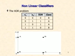
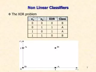
Non Linear Classifiers • The XOR problem
There is no single line (hyperplane) that separates class A from class B. On the contrary, AND and OR operations are linearly separable problems
The Two-Layer Perceptron • For the XOR problem, draw two, instead, of one lines
Then class B is located outside the shaded area and class A inside. This is a two-phase design. • Phase 1: Draw two lines (hyperplanes) Each of them is realized by a perceptron. The outputs of the perceptrons will be depending on the position of x. • Phase 2: Find the position of x w.r.t.bothlines, based on the values of y1, y2.
Equivalently: The computations of the first phase perform a mapping
The decision is now performed on the transformed data. This can be performed via a second line, which can also be realized by a perceptron.
Computations of the first phase perform a mapping that transforms the nonlinearly separable problem to a linearly separable one. • The architecture
This is known as the two layer perceptron with one hidden and one output layer. The activation functions are • The neurons (nodes) of the figure realize the following lines (hyperplanes)
Classification capabilities of the two-layer perceptron • The mapping performed by the first layer neurons is onto the verticesof the unit side square, e.g., (0, 0), (0, 1), (1, 0), (1, 1). • The more general case,
performs a mapping of a vector onto the vertices of the unit side Hp hypercube • The mapping is achieved with pneurons each realizing a hyperplane. The output of each of these neurons is 0 or 1 depending on the relative positionof x w.r.t. the hyperplane.
Intersections of these hyperplanes form regions in thel-dimensional space. Each region corresponds to a vertex of the Hp unit hypercube.
For example, the 001 vertex corresponds to the region which is located to the(-)side of g1(x)=0 to the(-)side of g2(x)=0 to the(+) side of g3(x)=0
The output neuron realizes a hyperplane in the transformed space, that separates some of the vertices from the others. Thus, the two layer perceptron has the capability to classify vectors into classes that consist of unions of polyhedral regions. But NOT ANYunion. It depends on the relative position of the corresponding vertices.
Three layer-perceptrons • The architecture • This is capable to classify vectors into classes consisting of ANY union of polyhedral regions. • The idea is similar to the XOR problem. It realizes more than one planes in the space.
The reasoning • For each vertex, corresponding to class, say A, construct a hyperplane which leaves THISvertex on one side (+) and ALLthe others to the other side (-). • The output neuron realizes an OR gate • Overall: The first layer of the network forms the hyperplanes, the second layer forms the regions and the output neuron forms the classes. • Designing Multilayer Perceptrons • One direction is to adopt the above rationale and develop a structure that classifies correctly all the training patterns. • The other direction is to choose a structure and compute the synaptic weights to optimize a cost function.
The Backpropagation Algorithm • This is an algorithmic procedure that computes the synaptic weights iteratively, so that an adopted cost function is minimized (optimized) • In a large number of optimizing procedures, computation of derivatives are involved. Hence, discontinuous activation functions pose a problem, i.e., • There is always an escape path!!! The logistic function is an example. Other functions are also possible and in some cases more desirable.
The steps: • Adopt an optimizing cost function, e.g., • Least Squares Error • Relative Entropy between desired responses and actual responses of the network for the available training patterns. That is, from now on we have to live with errors. We only try to minimize them, using certain criteria. • Adopt an algorithmic procedure for the optimization of the cost function with respect to the synaptic weightse.g., • Gradient descent • Newton’s algorithm • Conjugate gradient
The task is a nonlinear optimization one. For the gradient descent method
The Procedure: • Initialize unknown weights randomly with small values. • Compute the gradient terms backwards, starting with the weights of the last (3rd) layer and then moving towards the first • Update the weights • Repeat the procedure until a termination procedure is met • Two major philosophies: • Batch mode: The gradients of the last layer are computed once ALL training data have appeared to the algorithm, i.e., by summing up all error terms. • Pattern mode: The gradients are computed every time a new training data pair appears. Thus gradients are based on successive individual errors.
A major problem: The algorithm may converge to a local minimum
The Cost function choice Examples: • The Least Squares Desired response of the mth output neuron (1 or 0) for Actual response of the mth output neuron, in the interval [0, 1], for input
The cross-entropy This presupposes an interpretation of y and ŷ as probabilities • Classification error rate. This is also known asdiscriminative learning. Most of these techniques use a smoothed version of the classification error.
Remark 1: A common feature of all the above is the danger of local minimum convergence. “Well formed” cost functions guarantee convergence to a “good” solution, that is one that classifies correctly ALL training patterns, provided such a solution exists. The cross-entropycost functionis a well formed one.The Least Squaresis not.
Remark 2: Both, the Least Squares and the cross entropy lead to output values that approximate optimallyclass a-posteriori probabilities!!! That is, the probability of class given . This is a very interesting result. It does not depend on the underlying distributions. It is a characteristic of certain cost functions. How good or bad is the approximation, depends on the underlying model. Furthermore, it is only valid at the global minimum.
Choice of the network size. How big a network can be. How many layers and how many neurons per layer?? There are two major directions • Pruning Techniques: These techniques start from a large network and then weights and/or neurons are removed iteratively, according to a criterion.
Methods based on parameter sensitivity + higher order terms where Near a minimum and assuming that
Pruning is now achieved in the following procedure: • Train the network using Backpropagation for a number of steps • Compute the saliencies • Remove weights with small si. • Repeat the process • Methods based on function regularization
The second term favours small values for the weights, e.g., whereAfter some training steps, weights with small values are removed. • Constructive techniques:They start with a small network and keep increasing it, according to a predetermined procedure and criterion.
Remark: Why not start with a large network and leave the algorithm to decide which weights are small?? This approach is just naïve. It overlooks that classifiers must have good generalization properties. A large network can result in small errors for the training set, since it can learn the particular details of the training set. On the other hand, it will not be able to perform well when presented with data unknown to it. The size of the network must be: • Large enough to learn what makes data of the same class similar and data from different classes dissimilar • Small enough not to be able to learn underlying differences between data of the same class. This leads to the so called overfitting.
Overtraining is another side of the same coin, i.e., the network adapts to the peculiarities of the training set.
Generalized Linear Classifiers • Remember the XOR problem. The mapping The activation function transforms the nonlinear task into a linear one. • In the more general case: • Let and a nonlinear classification task. Also, let a number k of functions:
Are there any functions and an appropriate k, so that the mapping transforms the task into a linear one, in the space? • If this is true, then there exists a hyperplaneso that
In such a case this is equivalent with approximating the nonlinear discriminant function g(x), in terms of i.e., • Given , the task of computing the weights is a linear one. • How sensible is this?? • From the numerical analysis point of view, this is justified if are interpolation functions. • From the Pattern Recognition point of view, this is justified by Cover’s theorem
Capacity of the l-dimensional space in Linear Dichotomies • AssumeNpoints in assumed to be in general position, that is: Not of these lie on a dimensional space
Cover’s theorem states: The number of groupings that can be formed by (l-1)-dimensional hyperplanes to separate N points in two classes is Example:N=4, l=2, O(4,2)=14 Notice: The total number of possible groupings is24=16
Probability of grouping N points in two linearly separable classes is
Thus, the probability of havingNpoints in two linearly separable classes tends to 1, for large , providedN<2( +1) Hence, by mapping to a higher dimensional space, we increase the probability of linear separability, provided the space is not toodensely populated.
Radial Basis Function Networks (RBF) • Choose
Equivalent to a single layer network, with RBF activations and linear output node.
Example: The XOR problem • Define:
Training of the RBF networks • Fixed centers: Choose centers randomly among the data points. Also fix σi’s. Then is a typical linear classifier design. • Training of the centers: This is a nonlinear optimization task • Combine supervised and unsupervised learning procedures. • The unsupervised part reveals clustering tendenciesof the data and assigns the centers at the cluster representatives.
Universal Approximators It has been shown that any nonlinear continuous function can be approximated arbitrarily close, both, by a two layer perceptron, with sigmoid activations, and an RBF network, provided a large enough number of nodes is used. • Multilayer Perceptrons vs. RBF networks • MLP’s involve activations of global nature. All points on a plane give the same response. • RBF networks have activations of a local nature, due to the exponential decrease as one moves away from the centers. • MLP’s learn slower but have better generalization properties
Support Vector Machines: The non-linear case • Recall that the probability of having linearly separable classes increases as the dimensionality of the feature vectors increases. Assume the mapping: Then use SVM in Rk • Recall that in this case the dual problem formulation will be
Also, the classifier will be Thus, inner products in a high dimensional space are involved, hence • High complexity
Something clever: Compute the inner products in the high dimensional space as functions of inner products performed in the low dimensional space!!! • Is this POSSIBLE?? Yes. Here is an example Then, it is easy to show that
Mercer’s Theorem and let the inner product in H be given as Then for anyg(x), x: K(x,y)symmetric function known as kernel.