Signal Encoding Techniques

1. Signal Encoding Techniques Even the natives have difficulty mastering this peculiar vocabulary. —The Golden Bough, Sir James George Frazer

2. Signal Encoding Techniques

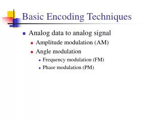
3. Digital Data, Digital Signal • digital signal • discrete, discontinuous voltage pulses • each pulse is a signal element • binary data encoded into signal elements

4. Terminology • unipolar – all signal elements have the same sign • polar – one logic state represented by positive voltage and the other by negative voltage • data rate – rate of data ( R ) transmission in bits per second • duration or length of a bit – time taken for transmitter to emit the bit (1/R) • modulation rate – rate at which the signal level changes, measured in baud = signal elements per second. • mark and space – binary 1 and binary 0

5. Key Data Transmission Terms

6. Interpreting Signals

7. Digital Signal Encoding Formats

8. Encoding Schemes

9. Nonreturn to Zero-Level(NRZ-L) • easiest way to transmit digital signals is to use two different voltages for 0 and 1 bits • voltage constant during bit interval • no transition (no return to zero voltage) • absence of voltage for 0, constant positive voltage for 1 • more often, a negative voltage represents one value and a positive voltage represents the other(NRZ-L)

10. Encoding Schemes

11. Non-return to Zero Inverted (NRZI) • Non-return to zero, invert on ones • constant voltage pulse for duration of bit • data encoded as presence or absence of signal transition at beginning of bit time • transition (low to high or high to low) denotes binary 1 • no transition denotes binary 0 • example of differential encoding • data represented by changes rather than levels • more reliable to detect a transition in the presence of noise than to compare a value to a threshold • easy to lose sense of polarity

12. NRZ Pros & Cons • used for magnetic recording • not often used for signal transmission

13. Multilevel BinaryBipolar-AMI • use more than two signal levels • Bipolar-AMI • binary 0 represented by no line signal • binary 1 represented by positive or negative pulse • binary 1 pulses alternate in polarity • no loss of sync if a long string of 1s occurs • no net dc component • lower bandwidth • easy error detection

14. Multilevel BinaryPseudoternary • binary 1 represented by absence of line signal • binary 0 represented by alternating positive and negative pulses • no advantage or disadvantage over bipolar-AMI and each is the basis of some applications

15. Multilevel Binary Issues • synchronization with long runs of 0’s or 1’s • can insert additional bits that force transitions • scramble data • not as efficient as NRZ • each signal element only represents one bit • receiver distinguishes between three levels: +A, -A, 0 • a 3 level system could represent log23 = 1.58 bits • requires approximately 3dB more signal power for same probability of bit error

16. Theoretical Bit Error Rate

17. Manchester Encoding • transition in middle of each bit period • midbit transition serves as clock and data • low to high transition represents a 1 • high to low transition represents a 0 • used by IEEE 802.3

18. Differential Manchester Encoding • midbit transition is only used for clocking • transition at start of bit period representing 0 • no transition at start of bit period representing 1 • this is a differential encoding scheme • used by IEEE 802.5

19. Biphase Pros and Cons

20. Spectral Density of Various Signal Encoding Schemes

21. Stream of Binary Onesat 1Mbps

22. Normalized Signal Transition Rate of Various Digital Signal Encoding Schemes Table 5.3  

23. Scrambling • use scrambling to replace sequences that would produce constant voltage • these filling sequences must: • produce enough transitions to sync • be recognized by receiver & replaced with original • be same length as original • design goals • have no dc component • have no long sequences of zero level line signal • have no reduction in data rate • give error detection capability

24. HDB3 Substitution Rules Table 5.4

25. B8ZS and HDB3

26. Digital Data, Analog Signal • main use is public telephone system • has frequency range of 300Hz to 3400Hz • uses modem (modulator-demodulator)

27. Modulation Techniques

28. Amplitude Shift Keying • encode 0/1 by different carrier amplitudes • usually have one amplitude zero • susceptible to sudden gain changes • inefficient • used for: • up to 1200bps on voice grade lines • very high speeds over optical fiber

29. Binary Frequency Shift Keying • two binary values represented by two different frequencies (near carrier) • less susceptible to error than ASK • used for: • up to 1200bps on voice grade lines • high frequency radio • even higher frequency on LANs using coaxial cable

30. Multiple FSK • each signalling element represents more than one bit • more than two frequencies used • more bandwidth efficient • more prone to error

31. FSK Transmission

32. Phase Shift Keying • phase of carrier signal is shifted to represent data • binary PSK • two phases represent two binary digits • differential PSK • phase shifted relative to previous transmission rather than some reference signal

33. DPSK

34. Bandwidth Efficiency for Digital-to-Analog Encoding Schemes

35. Quadrature PSK • more efficient use if each signal element represents more than one bit • uses phase shifts separated by multiples of /2 (90o) • each element represents two bits • split input data stream in two and modulate onto carrier and phase shifted carrier • can use 8 phase angles and more than one amplitude • 9600bps modem uses 12 angles, four of which have two amplitudes

36. QPSK and OQPSK Modulators

37. QPSK

38. Performance of Digital to Analog Modulation Schemes

39. Bit Error Rates for Multilevel FSK and PSK

40. Quadrature Amplitude Modulation • QAM used on asymmetric digital subscriber line (ADSL) and some wireless • combination of ASK and PSK • logical extension of QPSK • send two different signals simultaneously on same carrier frequency • use two copies of carrier, one shifted 90° • each carrier is ASK modulated • two independent signals over same medium • demodulate and combine for original binary output

41. QAM Modulator

42. QAM Variants • two level ASK • each of two streams in one of two states • four state system • essentially QPSK • four level ASK • combined stream in one of 16 states • have 64 and 256 state systems • improved data rate for given bandwidth • increased potential error rate

43. Analog Data, Digital Signal • digitization is conversion of analog data into digital data which can then: • be transmitted using NRZ-L • be transmitted using code other than NRZ-L • be converted to analog signal • analog to digital conversion done using a codec • pulse code modulation • delta modulation

44. Digitizing Analog Data

45. Pulse Code Modulation (PCM) • sampling theorem: • “If a signal is sampled at regular intervals at a rate higher than twice the highest signal frequency, the samples contain all information in original signal” • eg. 4000Hz voice data, requires 8000 sample per second • strictly have analog samples • Pulse Amplitude Modulation (PAM) • assign each a digital value

46. PCM Example

47. PCM Block Diagram

48. Non-Linear Coding

49. Typical Companding Functions

50. Delta Modulation (DM) • analog input is approximated by a staircase function • can move up or down one level () at each sample interval • has binary behavior • function only moves up or down at each sample interval • hence can encode each sample as single bit • 1 for up or 0 for down