Calibration and Editing George Moellenbrock
350 likes | 654 Vues
Calibration and Editing George Moellenbrock. Why calibration and editing? Formalism: Visibilities, signals, matrices Laundry List of Calibration Components Practical Calibration Planning Editing and RFI Calibration Sequence Examples Evaluating Calibration Performance Summary.

Calibration and Editing George Moellenbrock
E N D
Presentation Transcript
Calibration and EditingGeorge Moellenbrock Why calibration and editing? Formalism: Visibilities, signals, matrices Laundry List of Calibration Components Practical Calibration Planning Editing and RFI Calibration Sequence Examples Evaluating Calibration Performance Summary G. Moellenbrock, Synthesis Summer School, 18 June 2002
Why Calibration and Editing? • Synthesis radio telescopes, though well-designed, are not perfect (e.g., surface accuracy, receiver noise) • Need to accommodate engineering (e.g., frequency conversion, digital electronics, etc.) • Hardware or control software occasionally fails or behaves unpredictably • Scheduling/observation errors sometimes occur (e.g., wrong source positions) • Atmospheric conditions not ideal (not just bad weather) • RFI Determining instrumental properties (calibration) is as important as determining radio source properties G. Moellenbrock, Synthesis Summer School, 18 June 2002
From Idealistic to Realistic • Formally, we wish to obtain the visibility function, which we intend to invert to obtain an image of the sky: • In practice, we correlate the electric field (voltage) samples taken at pairs of telescopes (baselines i-j): • Single radio telescopes are devices for collecting the signal xi(t) and providing it to the correlator. G. Moellenbrock, Synthesis Summer School, 18 June 2002
What signal is really collected? • The net signal delivered by antenna i, xi(t), is a combination of the desired signal, si(t,l,m), corrupted by a factor Ji(t,l,m) and integrated over the sky, and noise, ni(t): • Ji(t,l,m) is the product of a host of effects which we must calibrate • In some cases, effects contained in the Ji(t,l,m) term corrupt the signal irreversibly and the resulting data must be edited • Ji(t,l,m) is a complex number • Ji(t,l,m) is antenna-based G. Moellenbrock, Synthesis Summer School, 18 June 2002
Aside: Correlation of signals • The correlation of two realistic signals from different antennas: • Noise doesn’t correlate—even if ni>> si, correlation isolates desired signals • In integral, only si(t,l,m), from the same directions correlate, so order of integration and signal product can be exchanged and terms re-ordered • …and the auto-correlation of a signal from a single antenna: • Desired signal not isolated from noise (less useful!) G. Moellenbrock, Synthesis Summer School, 18 June 2002
Formalism: Describe both polarizations via matrices • Need two polarizations (p,q) to fully describe sampled EM wave front, where p,q = R,L (circulars) or p,q = X,Y (linears) • Some components of Ji involve mixing of polarizations, so dual-polarization description desirable or even required • So substitute: • The Jones matrix thus corrupts a signal as follows: G. Moellenbrock, Synthesis Summer School, 18 June 2002
Signal Correlation and Matrices • Four correlations are possible from two polarizations. The outer product (a ‘bookkeeping’ product) forms them: • These four correlations (pp, pq, qp, qq) map to Stokes (I,Q,U,V) visibilities • A very useful property of outer products: • (where A,B,A’,B’ are matrices and/or vectors of appropriate dimensions): G. Moellenbrock, Synthesis Summer School, 18 June 2002
Signal Correlation and Matrices (cont) • The outer product for the Jones matrix: • Jij is a 4x4 Mueller matrix • Antenna and array design thankfully driven by minimizing off-diagonal terms G. Moellenbrock, Synthesis Summer School, 18 June 2002
Signal Correlation and Matrices (cont) • And finally, for fun, the correlation of corrupted signals: • UGLY, but let’s think about individual calibration components in the signal domain, where the matrices are a factor of 2 less complicated….. G. Moellenbrock, Synthesis Summer School, 18 June 2002
Calibration Components • Ji contains many components: • F= ionospheric Faraday rotation • T = tropospheric effects • P = parallactic angle • E = antenna voltage pattern • D = polarization leakage • G = electronic gain • B = bandpass response • Order of terms follows signal path • Each term has matrix form of Ji with terms embodying its particular algebra (on- vs. off-diagonal terms, etc.) • The full matrix equation (especially after correlation!) is daunting, but usually only need to consider the terms individually or in pairs, and rarely in open form (matrix formulation = shorthand) G. Moellenbrock, Synthesis Summer School, 18 June 2002
Ionospheric Faraday Rotation, F • The ionosphere is birefringent; one hand of circular polarization is delayed w.r.t. the other, introducing a phase shift: • Rotates the linear polarization position angle • More important at longer wavelengths: • More important at solar maximum and at sunrise/sunset, when ionosphere is most active • Beware of ‘patchiness’ and other variability (e.g., with elevation changes) • Namir’s lecture: “Long Wavelength Interferometry” (next Tuesday) G. Moellenbrock, Synthesis Summer School, 18 June 2002
Tropospheric Effects, T • The troposphere causes polarization-independent amplitude and phase effects due to emission/opacity and refraction, respectively • Typically 2-3m excess path length at zenith compared to vacuum • Most important at n > 15 GHz where water vapor absorbs/emits • More important nearer horizon where tropospheric path length greater • Clouds, weather = variability in phase and opacity; may vary across array • Water vapor radiometry? Phase transfer from low to high frequencies? • Claire’s lecture: “mm-Wave Interferometry” (next Monday) G. Moellenbrock, Synthesis Summer School, 18 June 2002
Parallactic Angle, P • Orientation of sky in telescope’s field of view • Constant for equatorial telescopes • Varies for alt-az-mounted telescopes: • Rotates the position angle of linearly polarized radiation (c.f. F) • Analytically known, and its variation provides leverage for determining polarization-dependent effects G. Moellenbrock, Synthesis Summer School, 18 June 2002
Antenna Voltage Pattern, E • Antennas of all designs have direction-dependent gain • Important when region of interest on sky comparable to or larger than l/D • Kumar’s lecture: “Wide Field Imaging I” (next Monday) • Debra’s lecture: “Wide Field Imaging II” (next Monday) • Important at lower frequencies where radio source surface density is greater and wide-field imaging techniques required • Beam squint: Epand Eq not parallel, yielding spurious polarization • For convenience, direction dependence of polarization leakage (D) may be included in E (off-diagonal terms then non-zero) G. Moellenbrock, Synthesis Summer School, 18 June 2002
Polarization Leakage, D • Polarizer is not ideal, so orthogonal polarizations not perfectly isolated • Well-designed feeds have d ~ a few percent or less • A geometric property of the feed design, so frequency dependent • For R,L systems, total-intensity imaging affected as ~dQ, dU, so only important at high dynamic range (because Q,U~d, typically) • For R,L systems, linear polarization imaging affected as ~dI, so almost always important • Greg’s lecture: “Polarization in Interferometry” (today!) G. Moellenbrock, Synthesis Summer School, 18 June 2002
Electronic Gain, G • Catch-all for most amplitude and phase effects introduced by antenna electronics (amplifiers, mixers, quantizers, digitizers) • Most commonly treated calibration component • Dominates other effects for standard observations • Includes scaling from engineering to radioastronomy units (Jy) • Often includes ionospheric and tropospheric effects which are typically difficult to separate unto themselves • Excludes frequency dependent effects (see B) G. Moellenbrock, Synthesis Summer School, 18 June 2002
Bandpass Response, B • G-like component describing frequency-dependence of antenna electronics, etc. • Filters used to select frequency passband not square • Optical and electronic reflections introduce ripples across band • Typically (but not necessarily) normalized G. Moellenbrock, Synthesis Summer School, 18 June 2002
More-sophisticated effects • Errors in geometric/clock models in correlator cause poor phase compensation • Routine problem in VLBI solved by fringe-fitting: parameterization of G to include phase terms which are linear in time and frequency • Craig’s lecture: “VLBI” (Thursday) • Baseline-based errors do not decompose into antenna-based components • Most digital correlators designed to limit such effects to well-understood and uniform scaling laws (absorbed in G) • Additional errors can result from averaging in time and frequency over variation in antenna-based effects and visibilities (practical instruments are finite!) • Correlated noise (e.g., RFI) • Virtually indistinguishable from source structure effects • Geodetic observers consider determination of radio source structure—a baseline-based effect—as a required calibration if antenna positions are to be determined accurately G. Moellenbrock, Synthesis Summer School, 18 June 2002
Putting it all back together • In the correlation of signals, like terms from the different antennas are conveniently grouped: • The total Measurement Equation has the form: • S maps the Stokes vector, I, to the polarization basis of the instrument • Mijand Aij are multiplicative and additive baseline-based errors, respectively • In general, all Jijmay be direction-dependent, so inside the integral…. G. Moellenbrock, Synthesis Summer School, 18 June 2002
Realizing practical calibration • …but in practice, we often ignore the direction dependence of the calibration components and factor them out of the integral (dropping Eij). The Measurement Equation then becomes a relation between the observed and ideal visibilities: • If the ideal visibilities are known (e.g., by choosing calibration source of known structure), we can solve for individual components using those we already know (if any), e.g.: G. Moellenbrock, Synthesis Summer School, 18 June 2002
Realizing practical calibration (cont) • Formally, solving for any component is the same non-linear fitting problem: • Algebraic particulars are stored safely and conveniently inside the matrix formalism (out of sight, out of mind!) • Viability of the solution relies on the underlying algebra (hardwired in calibration applications) and proper calibration observations • The relative importance of the different components enables deferring or even ignoring the more subtle effects G. Moellenbrock, Synthesis Summer School, 18 June 2002
Planning for Good Calibration • A priori calibrations (provided by the observatory) • Antenna positions, earth orientation and rate • Clocks • Antenna pointing, gain, voltage pattern • Calibrator coordinates, flux densities, polarization properties • Absolute calibration? • Very difficult, requires heroic efforts by visiting observers and observatory scientific and engineering staff • Cross-calibration a better choice • Observe nearby point sources against which calibration components can be solved, and transfer solutions to target observations • Choose appropriate calibrators for different components; usually point sources because we can predict their visibilities • Choose appropriate timescales for each component G. Moellenbrock, Synthesis Summer School, 18 June 2002
Calibrator Rules of Thumb • T, G: • Strong and point-like sources, as near to target source as possible • Observe often enough to track phase and amplitude variations: calibration intervals of up to 10s of minutes at low frequencies (beware of ionosphere!), as short as 1 minute or less at high frequencies • Observe at least one calibrator of known flux density at least once • B: • Strong enough for good sensitivity in each channel (often, T, G calibrator is ok) • If bandwidth is wide, should be point-like to avoid visibility changes across band • Observe often enough to track variations (e.g., waveguide reflections change with temperature and are thus a function of time-of-day) • D: • Best calibrator is strong and unpolarized • If polarized, observe over a broad range of parallactic angle to disentangle Dsand source polarization (often, T, G calibrator is ok) • F: • Choose strongly polarized source and observe often enough to track variation • If ionosphere is stable, rely on ionosonde observations for empirical corrections G. Moellenbrock, Synthesis Summer School, 18 June 2002
Data Examination and Editing • After observation, initial data examination and editing very important • Will observations meet goals for calibration and science requirements? • Some real-time flagging occurred during observation (antennas off-source, LO out-of-lock, etc.). Any such bad data left over? (check operator’s logs) • Any persistently ‘dead’ antennas (Ji=0 during otherwise normal observing)? (check operator’s logs) • Amplitude and phase should be continuously varying—edit outliers • Any antennas shadowing others? Edit such data. • Be conservative: those antennas/timeranges which are bad on calibrators are probably bad on weak target sources—edit them • Periods of poor weather? (check operator’s log) • Distinguish between bad data and poorly-calibrated data. E.g., some antennas may have significantly different amplitude response which may not be fatal—it may only need to be calibrated • Radio Frequency Interference (RFI)? • Choose reference antenna wisely (ever-present, stable response) G. Moellenbrock, Synthesis Summer School, 18 June 2002
A Data Editing Example • msplot in aips++ G. Moellenbrock, Synthesis Summer School, 18 June 2002
Radio Frequency Interference • RFI originates from man-made signals generated in the antenna or by external sources (e.g., satellites, cell-phones, radio and TV stations, etc.) • Obscures natural emission in spectral line observations • Adds to total noise power in all observations, thus decreasing sensitivity to desired natural signal, and complicating amplitude calibration • Though a contribution to the niterm, can correlate between antennas if of common origin or baseline short enough • RFI Mitigation • Careful electronics design in antennas • Observatories world-wide lobbying for spectrum management • Various on-line and off-line mitigation techniques under study • Choose interference-free frequencies (try to find 50 MHz of clean spectrum in the 1.6 GHz band!) • Observe continuum experiments in spectral-line modes so bad channels can be edited G. Moellenbrock, Synthesis Summer School, 18 June 2002
Radio Frequency Interference (cont.) • Growth of telecom industry threatening radioastronomy! G. Moellenbrock, Synthesis Summer School, 18 June 2002
Calibration Sequence I • Observation: total intensity spectral line imaging of weak target • A weak target source (1) • A nice near-by point-like G, T calibrator (2), observed alternately, but too weak for good B calibration (flux density unknown) • Three observations of strong flux density calibrator (3) which is also good for B calibration • Schedule (each digit is a fixed duration): 33-2-111-2-111-2-111-2-111-2-33-2-111-2-111-2-111-2-111-2-111-2-33 • Calibration sequence: • On 3, solve for G: • On 3, solve for B, using G: • On 2, solve for G, using B: • Scale 2’s Gs according to 3’s Gs: • Transfer B, G to 1: G. Moellenbrock, Synthesis Summer School, 18 June 2002
Calibration Sequence II • Observation: full-polarization imaging of weak target • A weak target source (1) • A nice, near-by, point-like, G, T calibrator (2), observed alternately, ok for D calibration, too (flux density and polarization unknown) • Three observations of strong flux density calibrator • Schedule (each digit is a fixed duration): 33-2-1111-2-1111-2-1111-2-1111-2-33-2-1111-2-1111-2-1111-2-1111-2-33 • Calibration sequence: • On 2 & 3, solve for G, using P: • Apply G to 2, get improved poln model: • On 2, solve for D, using P, G, & new model: • Scale 2’s Gs according to 3’s Gs: • Transfer D, G to 1, use P: G. Moellenbrock, Synthesis Summer School, 18 June 2002
Evaluating Calibration Performance • Are solutions continuous? • Noise-like solutions are just that—noise • Discontinuities indicate instrumental glitches • Any additional editing required? • Are calibrator data fully described by antenna-based effects? • Phase and amplitude closure errors are the baseline-based residuals; see Chapter 5 in book • Are calibrators sufficiently point-like? If not, self-calibrate: model calibrator visibilities (by imaging, deconvolving and transforming) and re-solve for calibration; iterate to isolate source structure from calibration components • Jim’s lecture: “Self-Calibration” (Wednesday) • Any evidence of unsampled variation? Is interpolation of solutions appropriate? • Self-calibration may be required, if possible G. Moellenbrock, Synthesis Summer School, 18 June 2002
G Solution Examples G. Moellenbrock, Synthesis Summer School, 18 June 2002
B Solution Examples G. Moellenbrock, Synthesis Summer School, 18 June 2002
Effect of Calibration on Visibility Data G. Moellenbrock, Synthesis Summer School, 18 June 2002
Effect of Calibration in the Image Plane Uncalibrated Calibrated G. Moellenbrock, Synthesis Summer School, 18 June 2002
Summary • Determining calibration is as important as determining source structure—can’t have one without the other • Data examination and editing and important part of calibration • Calibration dominated by antenna-based effects • Calibration formalism algebra-rich, but can be described piecemeal in comprehendible segments, according to well-defined effects • Calibration determination is a single standard fitting problem • Point sources are the best calibrators • Observe calibrators according requirements of components • Calibration sequences a juggling act of effects and corrections G. Moellenbrock, Synthesis Summer School, 18 June 2002