Linear and NonLinear Regression and Estimation Techniques
Linear and NonLinear Regression and Estimation Techniques. Course presentation EE-671 Presented by- Manesh Meena. Content. Introduction General Regression model Parameter estimation in LR Nonlinear and weighted Regression NARMAX modeling
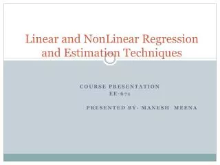

Linear and NonLinear Regression and Estimation Techniques
E N D
Presentation Transcript
Linear and NonLinear Regression and Estimation Techniques Course presentation EE-671 Presented by- ManeshMeena
Content Introduction General Regression model Parameter estimation in LR Nonlinear and weighted Regression NARMAX modeling Route training in mobile robotics through system identification Application of Regression analysis
Introduction • Regression analyses --to extract parameters from measured data, to define physical characteristics of a system. • Goal: Express the relationship between two (or more) variables by a mathematical formula. -x is the predictor (independent) variable -y is the response (dependent) variable We specifically want to indicate how y varies as a function of x.
Example • This can be understood from the following example • Consider a Car Loan Company • This company wants to predict behaviour of the costumers based on the previous historical behaviour .The data is is distributed as a narrow strip, and it is therefore possible to draw a curve that best "fits" the data . This curve will be considered as a satisfactory approximation of the true data distribution. • that is called the regression function of the variable "Budget" on the variable "Age". • Then using this regression function company will predict the value of the “Budget” attribute for the new customer.
Additional variables may be considered for the purpose of reducing the prediction errors on the predicted value of y. For example, Revenue, Gender, Annual milage, Number of children etc...could be included in the regression function. So, quite generally, doing regression is looking for the "best" function : y = f(x1, x2, ..., xp) • The regression function f(x1, x2, ..., xp) has therefore to be defined so as to make the prediction errors as small as possible. • Calculating Parameters There are two main ways of calculating the parameters of a regression model : • The "Least Squares" method, that minimizes the sum of the squares of the prediction errors of the model on the design data Simple and Multiple Regression models are adjusted by the Least Squares method. • The "Maximum Likelihood" method, that tunes the model so as to make the likelihood of the sample maximum.Logistic Regression models are adjusted by the Maximum Likelihood method.
General Regression Model • Assume the true model is of the form: y(x) = m(x) + ɛ(x) • The systematic part, m(x) is deterministic, • The error, ɛ(x) is a random variable -Measurement error -Natural variations due to exogenous factors Therefore, y(x) is also a random variable The error is additive • We want to estimate m(x) and possibly the distribution ɛ(x)
The Standard Assumptions • A1: E[ɛ(x)] = 0 ∀x (Mean 0) • A2: Var[ɛ(x)] = σ^2 ∀x • A3: Cov[ɛ(x), ɛ(x’)] = 0 ∀x ≠ x’ (Uncorrelated) These assumptions are only on the error term. ɛ(x) = y(x) − m(x) • Residuals • The residuals can be used to check the estimated model m’(x). • If the model fit is good, the residuals should satisfy our above three assumptions.
Parameter Estimation How to Estimate parameter m(x)?? Example: Relating Shoe Size to Height using footprint impressions
How can we estimate m(x) for the shoe example? • (Non-parametric): For each shoe size, take the mean of the observed heights. • (Parametric): Assume the trend is linear.
Linear Regression Simple linear regression assumes that m(x) is of the parametric form m(x) = β0 + β1x which is the equation for a line. Which line is the best estimate??
Write the observed data: yi = β0 + β1*xi + ɛi (i = 1, 2, . . . , n) Where yi ≡ y(xi) is the response value for observation i, β0 and β1 are the unknown parameters (regression coefficients), xi is the predictor value for observation i ɛi ≡ ɛ(xi) is the random error for observation i
Let g(x) ≡ g(x; β) be an estimator for y(x) Define a Loss Function L(y(x), g(x)) , which describes how far g(x) is from y(x) The Risk or expected loss is R(x)=E[L(y(x),g(x))] The best predictor minimizes the Risk (or expected Loss) g∗(x) = arg min E[L(y(x), g(x))] g∈G
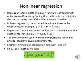
Non Linar Regression Nonlinear regression takes the general form y(x) = m(x; β) + ɛ(x) for some specified function m(x; β) with unknown parameters β. Making same assumptions as in linear regression (A1-A3), the least squares solution is still valid. Non-linear regression is an iterative procedure in which the number of iterations depend on how quickly the parameters converge.
Weighted Regression Consider the risk functions we have considered so far R(β) = ∑(yi − m(xi; β))^2 Each observation is equally contributes to the risk Weighted regression uses the risk function so observations with larger weights are more important
Nonlinear modeling To represent nonlinear models NARMAX(nonlinear autoregressive moving average with exazenous input) representation is used. For multiple input, single output noiseless systems, this model takes the form where y(n) and u(n) are the sampled output and input signals at time n respectively, Ng and Na are the regression orders of the output and input respectively. f() is a non-linear function.
Autoregressive moving average models The notation ARMA(p,q) refers to the model with p autorgressive terms and q moving average terms This model contains AR(p) and MA(q) models.
Nonlinear Autoregressive moving average with exozenous input(NARMAX) modeling The NARMAX methodology breaks the modeling problem into the following steps: 1.Structure Detection 2.Parameter Estimation 3.Model Validation 4.Prediction 5.Analysis
NARMAX Determine model structure and parameters based on estimation dataset. Validate the model using validation dataset. The initial structure of NARMAX polynomial is determined by the inputs u and output y and the input and the output time-lags Nu and Ng. The general rule in choosing the suitable inputs for the model is that at least some of them should be causing the output. But not all of them are significant contributors to the computation of the output. The final structure of the estimated NARMAX model will indicate only significant inputs.
NARMAX Before any removal of the model terms an equivalent auxiliary model is computed from the original NARMAX model. The model terms of the auxiliary model are orthogonal. The calculation of the auxiliary model parameters and refinement of the model’s structure is an iterative process. Each iteration involves three steps. 1. Estimation of model parameters using the estimation dataset. 2.Model validation using the validation dataset. 3.Removel of noncontributing terms.
NARMAX After the model validation step, if there is no significant error between the model predicted output and the actual output, non-contributing terms are removed in order to reduce the size of the polynomial. To determine the contribution of a model term to the output the Error Reduction Ratio (ERR) is computed for each term, which is the percentage reduction in the total mean-squared error as a result of including the term under consideration. Model terms with the ERR under certain threshold are removed from the model polynomial during the refinement process. In the following iteration if the error is higher as a result of last removal of the model term then these are reinserted back into the model and the model equation is considered as final. Finally NARMAX model parameters are computed from the auxiliary model.
Route Traning in mobile robotics through System Identification- Ulrich Nehmzow. • Purpose: to demonstrate how well the NARMAX model can represent route learning tasks. • Experimental procedure: • The robot is equipped with 16 sonar, 16 infra-red and 16 tectile sensors distributed uniformly around its circumference. • A sick laser range finder is also present which scans the front semi-circle of the robot with a radial resolution of 1 degree and distance resolution of 1 cm. • During experiment the inputs from all its sensors, its position, orientation, transitional and rotational velocities are recorded every 250 ms. • Position and orientation is obtained by placing point targets on top of the robot and using an overhead camera to track them continuously. • For the purpose of the experiment four separate route learning experiments were conducted.
Route Traning in mobile robotics through System Identification • In each case 1. initially the robot was driven manually several times through the specific route to be learned. 2. During this time robots sensor values and rotational velocities were logged. 3. The data collected was then used for estimation and validation of NARMAX model. 4. then the model was put on the robot and executed in order to record a further set of data that was used to test the model’s performance.
Route-1 After manual control for 1 hour all the sonar and laser measurements were taken. The values delivered by the laser scanner were averaged in 12 sectors of 15 degrees each(laser bins) to obtain a 12 dimensional vector of laser spaces. These laser bins as well as 16 sonar values were inverted so that large values indicate close-by-objects. Finally, the sonar and laser readings at each instant were normalized by minimum sonar and laser readings respectively at that instant. All these values are input into the model.
The parameters of the NARMAX model that author obtained were: • Nu=0, Ny=0, Ne=0, degree=2 • Initial model had 496 terms but after the removal of non-contributing terms only 70 remained. • To compare the two trajectories quantitatively difference between the distribution of values (x- x) under manual control and the distribution of the same under the NARMAX model was calculated which was not significant(~ 0.05).
Route-2 This time only laser sensor was used and pre-processed same as in route-1 The characteristics of the NARMAX model obtained are Nu=0, Ny=0, Ne=0 and degree=3. The initial model had 573 terms but just 94 remained after removal process of non-contributing terms. Statistical space occupancy tests along x and y axis confirms that there is no significant difference between the two trajectories(~.05)
Comparison Manual route-2 NARMAX route-2
Route-3 This time robot had to go through two narrow passes and many symmetries. To obtain the model normalized and inverted bins were used. The best NARMAX model uses Nu=0, Ny=0 and degree of polynomial=2. The initial model had 97 terms but after removal of non-contributing ones just 73 remained. Once again the model was properly able to learn the trajectory with no significant difference in the space occupancy.
Comparison Manual route-3 NARMAX route-3
Route-4 In this route robot had to start from position labelled A and had to reach to point labelled B. TO model the route’s behaviour ARMAX modeling was used which is the linear polynomial equivalent of NARMAX i.e. degree of polynomial is one. In this experiment regression order of output (Ny) was 0 and that of input(Nu) was 8. This model has successfully learned the route from A to B which was again confirmed using statistical analysis.
Applications of regression analysis Trend line analysis Risk analysis for investment Market forecasting Business Planning System Identification
References http://www.wikipedia.org/ http://dynsys.uml.edu/tutorials/regressionanalysis.htm “Route Training in mobile robotics: System Identification”- Ulrich Nehmzow and S. Billings
Questions • Type of the Model is linear or nonlinear? • How regression is different from correlation? • What will be the effect of adding polynomial terms in the Linear model? • What is the significance of coefficient of determination (R^2)? • What are the difficulties in regression analysis.?