Download
1 / 34
360 likes | 440 Vues
Explore crop growth and yield modeling techniques across different scales, from plots to regions, using dynamic agro-ecosystem models. Learn about statistical model approaches and a hybrid model for landscape scale analysis.

E N D
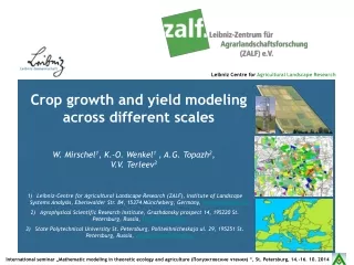
Crop growth and yield modeling across different scales W. Mirschel1, K.-O. Wenkel1 , A.G. Topazh2, V.V. Terleev3 • Leibniz-Centre for Agricultural Landscape Research (ZALF), Institute of Landscape Systems Analysis, Eberswalder Str. 84, 15374 Müncheberg, Germany, wmirschel@zalf.de • Agrophysical Scientific Research Institute, Grazhdansky prospect 14, 195220 St. Petersburg, Russia, topaj@hotmail.ru • State Polytechnical University St. Petersburg, Politekhnicheskaja ul. 29, 195251 St. Petersburg, Russia, vitaly_terleev@mail.ru
Content • Introduction • Dynamic agro-ecosystemmodel • 2.1 AGROSIM forplotscale • 2.2 AGROSIM for regional scale • Statistical modelapproaches • 3.1 Multiple nonlinearregressionforplotscale • 3.2 Cropyieldmodel YIELDSTAT for regional scale • Hybrid cropgrowthmodelforlandscapescale • Conclusions
Introduction (1) • Models are powerful tools for investigating the effects of different land use options and/or climate changes on agro-ecosystems as well as for bridging the gap between different temporal and spatial scales;they are urgentlyneeded to support ecological and economic conflict solutions. • Crop growth modeling at different spatial scales are very effective instruments for providing solutions to scientific, practical or impact assessment-oriented biomass and crop yield questions. • The best solution for both model developers and practitioners would be to havehighly resilient and robust universal crop growth models applicable to different questions and spatial scales. • BUT, experiences show that such a solution is hardly ever or never achieved in practice.The reality of crop growth modeling is that there is a close interaction between model type, spatial scale and input data availability.
Introduction (2) • Crop growth models require: ►meteorological values (Dj, j = 1, 2, ... nj); • ►management values (Mk, k = 1, 2,...nk); • ►site values (Sl, l = 1, 2, ... nl) and • ►parameters (Pm, m = 1, 2,... nm). • Xi = f [Dj, Mk, Sl, Pm] (Xi, i = 1,2,...ni) • At plot level all site and management conditions are well known; here detailed plant physiologic based crop growth models describing all important processes can be expected toproduce more scientific answers than similar simple crop growth approaches. • With increasing areas (from plot to region), there is a conflict between spatial heterogeneity, the heterogeneity in plant reaction patterns(local environ-mental conditions), the considered process details, and the input and parameter availability and uncertainty. • The selection of an model approach for the context depends on the modeling goal as well as realistic input and parameter demands so that accurate and resilient results can be achieved.
Dynamic agro-ecosystem model - AGROSIM for plot scale (1) - Model structure of AGROSIM models for winter cereals (dynamic process-based soil-plant-atmosphere-management model)
Dynamic agro-ecosystem model - AGROSIM for plot scale (2) - • The agro-ecosystemmodel AGROSIM: • describeshomogeneous crop stands under field conditions for limited water and nitrogen supply between sowing and harvest, • usesmeteorologicalstandardvalues(temperature, radiation, precipitation, CO2 content) asdrivingforces, • bases on availablesoilandmanagementinputvalues, • has a simularmodelstructurefor all crops, • uses rate equationsfordescribingprocessdynamics, • operates on a minimum time step of one day and • is sensitive to weather/climate, site and management. Model structure of AGROSIM models for winter cereals (dynamic process-based soil-plant-atmosphere-management model)
Dynamic agro-ecosystem model - AGROSIM for plot scale (3) - Validation of AGROSIM for German experimental sites in: Müncheberg, Hohenfinow, Ziethen, Mariensee, Bad Lauchstädt, Braunschweig Model-experiment comparison for ontogenesis, above-ground biomass and yield as time courses for the whole crop rotation (1993-1998) at the Müncheberg site (lines – simulations; squares – observations)
Dynamic agro-ecosystem model - AGROSIM for plot scale (4) - Validation of AGROSIM for Russian experimental sites in: Minkovo, Krasnodar, Sovetsk Krasnodar, 1983/84, variety: Mirinovskaja-808 Sovetsk, 1987/88, variety: Mirinovskaja-Jubiljenaja
Dynamic agro-ecosystem model - AGROSIM for plot scale (5) - Validation of AGROSIM for European experimental sites
Dynamic agro-ecosystem model - AGROSIM for plot scale (6) - problem with parametrization !!
Dynamic agro-ecosystem model - AGROSIM for regional scale (1) - The application of process-based agro-ecosystem models for the regional scale must be handled very carefully and is not possible in every case. However, in every case it is necessary to adapt these models to the practical cropping conditions taking into account the bias between the crop yield level for experimental stations and the crop yield level for practical cropping conditions. Two possibilities for usage of process-based agro-ecosystem models at regional scale: 1. Assumption that the region is a homogeneous area with homogenized model inputs, i.e. a typical soil for the whole region, a representative weather/climate data set for the region and a identical agro-management. 2. Sub-devision of the region into small grids (100m x 100m, for instance) there the model inputs can also be defined as homogeneous. The grid-based preparation of necessary model inputs for the whole region is much more difficult (problem: to acquire grid-based agro-management information ??)
Dynamic agro-ecosystem model - AGROSIM for regional scale (2) - 1. Example for first possibility with agro-ecosystem model AGROSIM Comparison of simulated and statistical average grain yields at district scale for Strausberg and Prenzlau districts in Brandenburg, Germany
Dynamic agro-ecosystem model - AGROSIM for regional scale (4) - Example for first possibility with agro-ecosystem model MONICA problem with limited weather stations !! 1992–2010 mean winter wheat yields in Thuringia, Germany, simulated on a 100 m × 100 m grid of soil and relief information with weather data from 14 weather stations following a nearest neighbour (Thiessen polygon) approach (Nendel et al., 2013)
Dynamic agro-ecosystem model - Problems for regional use (1) - • Main problems: • Dynamic models do not take into account all relevant processes and interactions influencing the biomass accumulation and yield formation. • Influences connected with infection pressure or with weed competition are not take into account. • Every cropandvarietyhasthereownparameterset. • Difference in cropyieldlevelbetween experimental plotsasbasis vor agro-ecosystemparametrizationandpracticalfieldcropping (ca. 10 … 20 %) • The cropyieldtrendbased on progress in plant breedingand agro-technology is not takenintoaccount. • Forusageon a regional scaletherearenecessary a large numberofinputdatarestrictionsandassumptions ( increasinguncertainty).
Statistical model approaches - Multiple nonlinear regression for plot scale - BM - above-ground biomass, x1 - field capacity of growing site, x2 - soil moisture at sowing, x3 - temperature sum above 0 °C, x4 - sum of global radiation, x5 - sum of precipitation Model-Experiment-Comparison for winter wheat above-ground total biomass (Müncheberg, Hohenfinow and Ziethen, 1991-1997, R2 = 0.9381, MABS = 81.44 g m-2)
Statistical model approaches - Crop yield model YIELDSTAT for regional scale (1) - Matrix for basic natural yield (YBY) for: - 56 site types - 16 different agricultural crops - 2 grassland-types (intensive, extensive) Basis: field-specific yield data from about 300 farms during a period of 15 years Site-specific yield extra charges (+ , - ) YSite= f (slope, stoniness, altitude, hydromorphy, soil quality index, climate zone, crop growth temperature, average winter temperature, climatic water balance, …) Soil tillage effect YSoTi = f(soil type, soil tillage method, crop type, pre-crop) Basis: soil tillage experiments Pre-crop effect YPrCr = f(current crop, pre-crop) Basis: crop rotation experiments Progress in plant breeding and agro-technology YTech = f (cropping year,level of plant breeding, level of agro- management) Basis: long-term yield statistics, trend prediction CO2-effect fCO2 = f (crop species (C3, C4), cropping year, atmospheric CO2) Basis: FACE-, open-top and climate chamber experiments Irrigation effect YIrri = f (irrgation water demend, water use efficiency) Basis: irrigation experiments Yield loss by advers weather conditions YLoHa = f(main harvest month, precipitation) Basis: yield statistics, weather statistics
Statistical model approaches - Crop yield model YIELDSTAT for regional scale (2) - Matrix for basic natural yield (YBY) for: - 56 site types - 16 different agricultural crops - 2 grassland-types (intensive, extensive) Basis: field-specific yield data from about 300 farms during a period of 15 years Site-specific yield extra charges (+ , - ) YSite= f (slope, stoniness, altitude, hydromorphy, soil quality index, climate zone, crop growth temperature, average winter temperature, climatic water balance, …) Soil tillage effect YSoTi = f(soil type, soil tillage method, crop type, pre-crop) Basis: soil tillage experiments Pre-crop effect YPrCr = f(current crop, pre-crop) Basis: crop rotation experiments Progress in plant breeding and agro-technology YTech = f (cropping year,level of plant breeding, level of agro- management) Basis: long-term yield statistics, trend prediction CO2-effect fCO2 = f (crop species (C3, C4), cropping year, atmospheric CO2) Basis: FACE-, open-top and climate chamber experiments Irrigation effect YIrri = f (irrgation water demend, water use efficiency) Basis: irrigation experiments Yield loss by advers weather conditions YLoHa = f(main harvest month, precipitation) Basis: yield statistics, weather statistics Y = ((YBY + YSite) · fPrCr · fTill + YTech) · fCO2 + YIrri − YLoHa
Statistical model approaches - Crop yield model YIELDSTAT for regional scale (9) - Spatial Analysis and Modeling Tool (SAMT) Maps (Thuringia, Germany) [Wieland et al., 2006] Soil index Thuringia, Germany Data base (Weather/Climate, Parameter, Management) Altitude Hydromorphy Soil type Climate zoning Model Grids: 100m x 100m (1 ha) Hybrid model YIELDSTAT Szenario simulations for Silage maize Crop yield Irrigation water demand
Statistical model approaches - Crop yield model YIELDSTAT for regional scale (10) - Crop yield changes 2021-2050 vs. 1981-2010 (%, regionalized for the Free State of Thuringia, Germany) Winter wheat Spring barley Winter rape Silage maize
Hybrid crop growth model for landscape scale (1) Within agro-landscapes, crop growth models are necessary for different agricultural crops and grassland types as well as for different management intensities (Germany: ca. 20 arable crops, 14 grassland types) Limited availability of input data at landscape scale - GIS-based data with different spatial resolutions (soil maps, land use maps…) - no specific management information - no specific cultivar information - weather/climate information based on the official weather service station network only - … Here the usage of dynamic plant-physiological-based agro-ecosystem models is not optimal, i.e. is connected with a lot of problems ! Solution: a hybrid crop growth model which include sub models of different approaches (statistics, fuzzy, neural network, empirical approach and others)
Hybrid crop growth model for landscape scale (3) Structure of a generic hybrid model for crop growth
Hybrid crop growth model for landscape scale (4) YIELDSTAT Mirschel et al. (2014)
Hybrid crop growth model for landscape scale (5) EVOLON approach Peschel (1988)
Hybrid crop growth model for landscape scale (6) PET= (G + K) (T + 22)/(150 (T + 123)) T ‑ daily mean temperature (°C) G ‑ daily radiation (J cm‑2) K ‑ constant Wendling et al. (1991)
Hybrid crop growth model for landscape scale (7) ONTO (1975 (inside) vs. 2040 (outside)) Mirschele et al. (2010)
Hybrid crop growth model for landscape scale (8) BOWET Mirschel et al. (1995)
Conclusions Because of required model simplifications on the one hand and increasing difficulties in the process of input data availabilityconnected with increasing scales on the other, it follows thatthere is a mutual dependency between scale and applied model type for crop growth. It is unwise to search for an optimum modeling approach that can be used across all scales.Instead,it is advisable to find the best suitable modeling approach according to the scale of the project. In order to obtain resilient and robust results in crop growth modeling on a large scale across a wide range of agricultural crops grown on arable and grass land, it is recommended that hybrid crop growth models are used which combine different statistical, matrix, fuzzy and expert knowledge -based approaches with empirical algorithms. The special challenge in crop growth modeling is to find a balance between the modeling goal, the input data availability (including quantity and quality), the spatial scale, and the model type.
Statistical model approaches - Crop yield model YIELDSTAT for regional scale (3) - Basic natural yield matrix (YBY) StT - soil type NY - natural yield (t ha-1) WW - winter wheat TR - triticale
Statistical model approaches - Crop yield model YIELDSTAT for regional scale (4) - Crop type specific yield extra charges as function of site specific characteristics (here for winter rape) YSite + 0.02 KWBJ-A • StT – site type (V – disintegrated type) • KWB – climatic water balance during vegetation (mm) • KWBJ-A – climatic water balance forJune – August (mm) • KlZ – mesoscalic climatic zone • HaNe – slope steepness (%) • SK - stoniness (t/ha) • AZ – soil quality index • HüNN - altitude (m) • Hy – hydromorphy class • WaWiT – groth temperature threshold
Statistical model approaches - Crop yield model YIELDSTAT for regional scale (5) - Yield effects - of previous crops (fPrCr) - of soil tillage (fTill)
Statistical model approaches - Crop yield model YIELDSTAT for regional scale (6) - Crop yield trend caused by progress in plant breeding and agro-technology Crop yield trend estimation for the Free State of Thuringia Declining crop yield trends (dt ha-1 a-1) for the Free State of Thuringia, Germany, for the time period up to 2050 started from the real yield trends for 1991-2010
Statistical model approaches - Crop yield model YIELDSTAT for regional scale (7) - Yield effect of rising atmospheric CO2 fCO2(FA) - ffactor of complex impact of CO2 on yield FA - crop type CO2(KlSz, J) – atmospheric CO2-content J – year of simulation KlSz - climate scenario used CO2Eff - efficiency factor (% per 1 ppm CO2 increase) KWB - climatic water balance (mm) for the FA-dependent vegetation year Effectiveness of a atmospheric CO2-increase on biomass accumulation of agricultural crops [% (1ppm CO2-increase)-1] based on results from the „Centre for the Study of Carbon Dioxide and Global Change“ (2009)
Statistical model approaches - Crop yield model YIELDSTAT for regional scale (8) - Yield losses by adverse weather situations during harvest time EV -yield loss (dt ha-1); NiTage -number of days with precipitation > 0 mm during harvest periode; miNiTage -long-term average of number of days with precipitation during harvest period; Ni∑ -precipitation sum during harvest period (mm); miNi∑ -long-term average of precipitation sum during harvest period (mm); maNi∑ -max. precipitation sum during harvest period (mm); A, B, C, D -statistical parameters Crop type dependent parameter values for the yield loss algorithm