Download

1 / 32
431 likes | 952 Vues
Control theory explores the behavior of dynamical systems and the mechanisms needed to maintain desired outputs. In applications such as air conditioning, controllers manipulate inputs based on error signals generated from the difference between actual and desired outputs (set-points). The ON-OFF control method turns systems on or off based on set-points with hysteresis to avoid unnecessary fluctuations, while PID (Proportional-Integral-Derivative) control offers a more nuanced approach, adjusting outputs based on current errors, accumulated past errors, and error rates.

E N D
ON-OFF & PID Controllers
ControlTheory Control theory deals with the behavior of dynamical systems. The desired output of a system is called the reference or set-point. When an output variable of a system need to follow a certain reference over time, a controller is required to manipulate the input to obtain the desired effect on the output of the system. In air conditioning systems a feedback loop control is usually implemented. This is a negative feedback, because the sensed value is subtracted from the desired value to create the error signal which is amplified by the controller. Controller System Sensor Set-Point Error Input Output + -
ControlTheory The controller also faces with disturbances coming from the surrounding environment and from the electronic equipments. SN System Sensor LN Controller Load Noise + Set-Point Error Input Output + + - + + Sensor Noise
Typesof Controller • Let consider the problem to heat a room till a desired temperature (set-point) by using an electrical heater. • We can control the heating through two different ways: • Switching on and off the heater. • Modulating the heating power. Heating set-point 100 % 0 % ON HEATER OFF Temperature [°C]
ON-OFF Control The easiest way to control the system is the ON-OFF control. It follows the law: Heating set-point ON HEATER OFF Temperature [°C]
ON-OFF Control REAL ON-OFF CONTROL (with hysteresis and dead zone) IDEAL ON-OFF CONTROL set-point set-point ON ON - OFF OFF Controlled Variable Controlled Variable
ON-OFF Control When the room temperature is lower than the set-point, the heater is turned on at maximum power, and once the room temperature is higher than the set-point, the heater is switched off completely. The turn-on and turn-off temperatures differ by a small amount, known as hysteresis, which prevent noise from switching the heater rapidly and unnecessarily when the temperature is near the set-point. The fluctuations in temperature are significantly larger than the hysteresis, due to the significant heat capacity of the heating element. output set-point Temperature [°C] Hysteresis ON OFF Power Time [s]
PID Control Set-Point Error Input Output + - Sensor D I P Controller System Controller • PID control divides into 3 actions: • Proportional • Integral • Derivative + Error Input + +
PID Control Set-Point Error Input Output Sensor P System D I + - Heating set-point 100 % + + + 0 % Temperature [°C]
PID Control • The Proportional value determines the reaction to the current error; • The Integral value determines the reaction based on the sum of recent errors; • The Derivative value determines the reaction based on the rate at which the error has been changing. • The weighted sum of these three actions is used to adjust the process via a control element such as the power supply of a heating element or the position of a control valve. • By "tuning" the three constants in the PID controller algorithm, the controller can provide control action designed for specific process requirements. The response of the controller can be described in terms of the sensitiveness of the controller to an error, the degree to which the controller overshoots the set-point and the degree of system oscillation.
ProportionalAction The proportional action makes a change to the output that is proportional to the current error value. The proportional response can be adjusted by multiplying the error by a constant K, called the proportional gain. The proportional action is given by: where: P Proportional term of output K Proportional gain (tuning parameter) e Error = set-point − previous value t Instantaneous time A high proportional gain results in a large change in the output for a given change in the error.
ProportionalAction If the proportional gain is too high, the system can become unstable. In contrast, a small gain results in a small output response to a large input error, and a less sensitive controller. If the proportional gain is too low, the control action may be too small when responding to system disturbances. A pure proportional control will not settle at its target value, but will retain a steady state error that is a function of the proportional gain and the process gain. Despite the steady-state offset, it is the proportional term that contribute the bulk of the output change. Temperature [°C] Time [s]
IntegralAction The integral action is proportional to both the magnitude of the error and the duration of the error. The addition of the instantaneous error over time (integrating the error) gives the accumulated offset that should have been corrected previously. The accumulated error is then multiplied by the integral time and added to the controller output. The magnitude of the contribution of the integral term to the overall control action is determined by the integral time, Ti. The integral action is given by: where: I Integral term of output Ti Integral time (tuning parameter) e Error = set-point − previous value t Time in the past contributing to the integral response
IntegralAction The integral action (when added to the proportional action) accelerates the movement of the process towards the set-point and eliminates the residual steady-state error that occurs with a proportional only controller. However, since the integral term is responding to accumulated errors from the past, it can cause the present value to overshoot the set-point value (cross over the set-point and then create a deviation in the other direction). Temperature [°C] Time [s]
Derivative Action The rate of change of the process error is calculated by determining the slope of the error over time (its first derivative with respect to time) and multiplying this rate of change by the derivative time Td. The magnitude of the contribution of the derivative action to the overall control action is termed the derivative time, Td. The derivative action is given by: where: D Derivative term of output Td Derivative time (tuning parameter) e Error = set-point − previous value t Instantaneous time
Derivative Action The derivative term slows the rate of change of the controller output and this effect is most noticeable close to the controller set-point. Hence, derivative control is used to reduce the magnitude of the overshoot produced by the integral component and improve the combined controller-process stability. However, differentiation of a signal amplifies noise and thus this term in the controller is highly sensitive to noise in the error term, and can cause a process to become unstable if the noise and the derivative time are sufficiently large. Temperature [°C] Time [s]
P+I+D Actions Error e(t) System input u(t) The proportional, integral, and derivative actions are added to calculate the output of the PID controller. Defining u(t) as the system input, the final form of the PID algorithm is: and the tuning parameters are: K: Proportional gain – larger K typically means faster response. The larger the error, the larger the proportional term compensation. An excessively large proportional gain will lead to process instability and oscillation. Ti: Integral time – larger Ti implies steady state errors are eliminated quicker. It causes larger overshoot: any negative error integrated during transient response must be integrated away by positive error before we reach steady state. Td: Derivative time – larger Td decreases overshoot, but slows down transient response and may lead to instability due to signal noise amplification in the differentiation of the error.
PID adjustment While designing a PID controller for a given system, follow the steps shown below to obtain the desired response. Add a proportional control to improve the rise time; Add an integral control to eliminate the steady-state error; Add a derivative control to improve the overshoot; Adjust each of K, Ti, and Td until you obtain the desired overall response. Keep in mind that you do not need to implement all three controllers (proportional, derivative and integral) into a single system, if not necessary. For example, if a PI controller gives a good enough response, then you don't need to implement derivative controller to the system. Keep the controller as simple as possible.
PID adjustment A proportional controller (K) will have the effect of reducing the rise time and will reduce, but never eliminate, the steady-state error. An integral control (Ti) will have the effect of eliminating the steady-state error, but it may make the transient response worse. A derivative control (Td) will have the effect of increasing the stability of the system, reducing the overshoot and improving the transient response. Effects of each of controllers K, Ti and Td on a closed-loop system are summarized in the table shown below: Note that these correlations may not be exactly accurate, because K, Ti and Td are dependent of each other. In fact, changing one of these variables can change the effect of the other two. For this reason, the table should only be used as a reference when you are determining the values for K, Ti and Td.
ON-OFF & PID Simulations CLICK ON THE ICON TO START EXCEL SIMULATION
UniflairControlTechniques CHILLED WATER UNITS (CW)
UniflairControlTechniques DIRECT EXPANSION UNITS (DX)
UniflairControlTechniques TWIN COOL UNITS (TC)
UniflairControlTechniques ENERGY SAVING UNITS (ES)
UniflairControlTechniques HUMIDIFICATION AND DEHUMIDIFICATION
UniflairControlTechniques AUTOADAPTATIVE HYSTERESIS ON ARA UNITS