Download
1 / 27
290 likes | 513 Vues
This handout explores the quantum measurement problem, focusing on the entangled "measurement state" of a qubit system during an ideal, non-disturbing measurement. It discusses the implications of Einstein's causality and the need for local mixtures of the states involved. The paper addresses contradictions inherent in instantaneous collapse and proposes a solution involving local collapse that aligns with established quantum principles and experimental confirmations. A brief history of non-locality and insightful experiments clarify the nature of measurement in quantum mechanics.

E N D
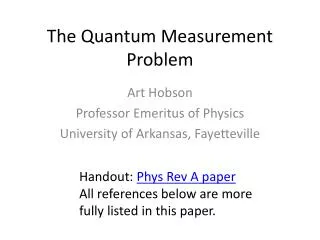
The Quantum Measurement Problem Art Hobson Professor Emeritus of Physics University of Arkansas, Fayetteville Handout: Phys Rev A paper All references below are more fully listed in this paper.
ABSTRACT In an ideal (non-disturbing) measurement of a qubit (2-state) system S by an apparatus A, S & A are put into an entangled“measurement state.” Because entangled states are non-local, the requirement of Einstein causality implies all local (at either S or A) observations to be fully described by local mixtures of the states of S or the states of A. These local mixed states are incoherent, and exhibit definite eigenvalues—definite outcomes such as “alive” or “dead” for Schrodinger’s cat—with no superposition or interference. However, S and A are not actually in the corresponding eigenstates—they are in the measurement state. Thus, the standard eigenvalue-eigenfunction link is broken. Macroscopic observation (which destroys the coherent measurement state) preserves the mixture, revealing a definite (but unpredictable) outcome.
Outline I. What’s the problem? II. An enlightening experiment. III. A proposed solution to the problem.
I. WHAT’S THE PROBLEM? • Consider a qubit system S, Hilbert space HSspanned by |s1>, |s2>. • Superposition |𝜓>S = α|s1> + β|s2>. • Apparatus A “measures” S, obtaining a “definite outcome” (eigenvalue) s1 or s2. • Measurement postulate: S “collapses” instantly into either |s1> or |s2>. • The problem: If the world obeys Q physics, we should be able to derive this collapse from Sch. eq. for A and S. How to do this?
Setting up the problem: • Assume A has states |ready>, |a1>, |a2> ∊ HA such that: |ready>|s1>→|a1>|s1> and |ready>|s2>→|a2>|s2> --“ideal non-disturbing meas.” • Linearity of the Schrodinger evolution implies |ready>|𝜓>S→ α|a1>|s1> + β|a2>|s2>
Apparent contradictions: • |𝚿> = α|a1>|s1> + β|a2>|s2> (measurement state) appears to describe a superposition of SA with superposed states |a1>|s1> & |a2>|s2> --a macro superposition! Ex: Schroedinger’s cat. • Where’s the collapse, to |a1>|s1> or |a2>|s2>? • Furthermore, such a collapse would be non-linear, which contradicts Sch’s eq. • Furthermore, the collapse postulate says collapse is instantaneous. Many experts think changes such as |𝚿>→|a1>|s1> can’t be instantaneous. • So most experts think the problem isn’t solvable, and major foundational changes are needed.
Some history: • John von Neumann, 1932, saw the problem. • Erwin Schrodinger, 1935, formulated it as Sch’s cat. • My proposal (below) is similar to 3 previous proposals: --Marlan Scully, Shea, McCullen, 1978. --Marlan Scully, Englert, Julian Schwinger, 1989. --Rinner & Werner, 2008. • Also, the “modal interpretation” (David Dieks et al) is similar to my proposal--but it postulates this solution rather than deriving it from Q physics and experiment. • There are also MANY proposed “interpretations”that claim to resolve the problem! Many worlds etc.
A proposed solution: “Local collapse” • Follows from conventional QP with no need for a measurement postulate, and is (IMO) confirmed by experiments. • It’s not a new interpretation. • It requires no new physics, e.g. a “collapse mechanism.” • The key: A close look at the measurement state, especially its non-local properties. • The results imply revising the “eigenfunction/eigenvalue link” (discussed later).
II. AN ENLIGHTENING EXPERIMENT. • Measurement State (MS): |𝚿> = α|a1>|s1> + β|a2>|s2> • An entangled superposition of two subsystems A & S. • They are non-locally connected (Gisin, 1991). • This non-locality makes it quite different from a simple superposition such as |𝜓>S= α|s1> + β|s2>. • The MS is commonly viewed as a superposition of two states, |a1>|s1> & |a2>|s2>, of a composite system SA. • But experiment (and analysis) show: The MS must be viewed as a superposition of two non-local correlations, in which |a1> is corr with |s1> and|a2> is corr with |s2>.
Brief history of non-locality • Einstein (Solvay Conf 1927) was the first to note that the collapse postulate implies non-locality. • Einstein developed this in his “EPR” paper (1935), used it to argue against std QP. • John Bell (1964) derived an inequality involving correlated outcomes of experiments on two systems; violation of the inequality implied the systems to be non-locally related; quantum physics violates Bell’s inequality in certain cases. • John Clauser(1972) and Alain Aspect (1982) performed exps with entangled photon polarizations to test whether QP, or locality (Bell’s inequality), were correct. QP won. • The results showed that, regardless of QP, nature is non-local. • Aspect’s exp showed non-local corrs are estab “faster than c.”
Exp of Rarity/Tapster, &Ou et al (RTO) 1990. Two entangled photons, A & S. The exp, which used beam splitters, variable phase shifters, and photon detectors, is equivalent to the following 2-photon double slit exp:
mirror mirror y path s2 path a1 photon A photon S Source of two entangled photons x path s1 path a2 mirror mirror With no entanglement, this would be two 2-slit exps: states (|a1>+|a2>)/√2 and (|s1>+|s2>)/√2. Interference fringes at both screens. With entanglement, the state is the MS! |𝚿> = (|a1>|s1> + |a2>|s2> )/√2. Each photon measures the other! The exp is a probe of the MS, with variable phases!
Results of RTO exp: • In a series of trials, neither A’s screen nor S’s screen shows any sign of interference or phase dependence: x & y are distributed randomly all over A’s & S’s screen. • The reason: Each photon acts as a “which path” detector for the other photon. • A is either in state |a1> (upper slit) or state |a2> (lower slit). Similarly for S. • Each photon is in an incoherent “mixture,” rather than a coherent superposition.
Wheredoes the coherence go? y-x is proportional to the difference of the two phases 𝝋A - 𝝋S. • --It can’t vanish, because the Schrodinger evolution is “unitary.” • Ans: the correlations become coherent: When coincidences of entangled pairs are detected at A’s and S’s screens: coincidence rate ∝cos(𝝋A - 𝝋S) = cos(y-x). • Photon A strikes it’s screen randomly at x, and photon S then strikes its screen in an interference pattern around x! & vice-versa. • This certainly seems non-local, and in fact the results violate Bell’s inequality.
What are “coherent correlations”? 𝝋A-𝝋S=0, 2π, 4π When 𝝋A-𝝋S=0, 2π, …, A and S are correlated: ai occurs iffsi occurs. When 𝝋A-𝝋S=π, 3π, 5π, ..., A and S are anti- corr: ai occurs iffsi does not occur. When 𝝋A-𝝋S=π/2, 3π/2, 5π/2, …, A and S are not at all correlated. This is an interference of correlations between states, rather than the usual single-photon interference of states.
It’s an important conclusion: • The MS |𝚿> = α|a1>|s1>+β|a2>|s2> is not a state in which either S or A interferes with itself. Instead, it’s a superposition only of the correlations between S and A.
Bell’s theorem implies…. …that the results are truly non-local: Cannot be explained by “prior causes” or by “causal communication.” Thus, if S’s phase shifter changes, the outcomes on A’s (and S’s) screen are instantly altered. Aspect’s exp tested these predictions (but with photon polarizations): The results confirmed violation of Bell’s ≠ and the observed changes showed up at the distant station sooner than a lightbeam could have gotten there.
III. A proposed solution to the meas. prob. • Density operator format: Expected values of observables Q can be found from the “density operator” ρ = |𝚿> <𝚿| (where|𝚿> = MS) from 〈Q〉 = TrSA(ρQ). • For observables QS ∊ HS , 〈QS〉 = TrS(ρSQS) where ρS =“reduced density operator for S alone” = TrAρ = <a1|ρ|a1> + <a2|ρ|a2> = |s1> |α|2 <s1| + |s2> |β|2 <s2|
Entanglement has “diagonalized” the density op for S: • Before entanglement, |𝜓>S = α|s1> + β|s2>, ρSbef = |𝜓>SS<𝜓| = ⎡|α|2 αβ* ⎤ ---coherent. ⎣α*β |β|2 ⎦ • After entanglement, ρS =TrA(|𝚿> <𝚿|) = ⎡|α|2 0⎤ ---incoherent, ⎣0 |β|2⎦ mixed state • Entanglement has “decohered” photon S. • Photon S no longer interferes with itself. The interference (coherence) has been transferred to an interference between the S-A correlations.
Are ρS and ρA the collapsed states we expect? •ρS predicts that a “local” observer (an obs of S alone) will observe either |s1> or |s2>, not a superposition (Sch’s cat: either an undecayed or decayed nucleus, not both). • ρApredicts that a local observer of A will observe either|a1> or|a2>, not a superposition (either an alive cat or a dead cat, not both). • This sounds promising. • In fact, it’s been hailed as the solution by Scully-Shea-McCullen 1978, Scully-Englert-Schwinger 1989, Rinner-Werner 2008, and the modal interp of Dieks and others.
But many experts have two objections First: “basis ambiguity”: If |α|2=|β|2 then the eigenvalues of ρS &ρA are equal and their eigenvectors are ambigious. • In fact, ρS=IS/2 and ρA=IA/2 where IS and IA are identity ops. The bases for ρS and ρA could be any orthonormal set, e.g. (|s1>±|s2>)/√2. • Answer:This happens onlyfor the special case |α|2=|β|2, e.g. only when t = halflife of Sch’s nucleus. For the general case, there’s no ambiguity. • More fundamentally: The basis for the physical problem is determined by the experimental arrangement. Apparatus A detects states |s1> and |s2>--not |s1>±|s2>--via apparatus states |a1> and |a2>.
Second objection: • ρS and ρA are “improper density ops.” • --Because they do not represent ignorance of the actual state. • That is, ρS=|s1>|α|2<s1|+|s2>|β|2<s2| does not represent a situation in which “S is in |s1> with probability |α|2 and in |s2> with probability |β|2,” because S is in fact in the MS! • This “ignorance interpretation” is the usual way of viewing incoherent or mixed states.
However, ρS and ρAmust yield the correct observations at S and A. Here’s why: • S and A are entangled, thus non-locally connected. • Thus all info about S-A correlations must be “camouflaged from” local observers of S & A. The reason: If an observer could, by observing S alone, detect any change when 𝛗A is changed, A could send an instant signal to S across an arbitrary distance. • SR (Einstein causality) does not allow this. • In fact Ballentine 1987 and Eberhard 1989 have shown that quantum probabilites do just what’s needed: When A alters φA, only the correlations change—the statistics of the outcomes at S don’t change. • This protection of Einstein causality is a remarkable and delicate feature of quantum entanglement.
Continuing this argument, let’s return to the MS |𝚿> = α|a1>|s1>+β|a2>|s2>. • The MS contains three kinds of info: (1) “Local info” about observations of S alone. (2) “Local info” about observations of A alone. (3) “Non-local info” about S-A correlations. • (1) is entirely described by ρS. • (2) is entirely described by ρA. • We’ve seen that “local” observations of S alone or of A alone cannot provide access to (3). • Conclusion: ρS and ρAmust represent precisely the observations of the local observers. • Example: Schrodinger’s cat must be either alive or dead, not both.
This resolves the “problem of outcomes”--the question of how a definite outcome arises when A measures S. • The standard principles of QP imply that definite outcomes are observed when A measures S. • But we have not derived the postulated collapse. This postulate says: the MS collapses to either |s1>|a1> or |s2>|a2>. We have shown, instead, that A and S exhibit definite eigenvalues si and ai (i=1 or 2). S & A are not in the corresponding eigenstates—they are in the MS. • Thus we have not yet justified the collapse postulate—we have shown that when A measures S, a definite eigenvalue s1 or s2 (e.g. “undecayed” or “decayed”) is observed, but we have not shown that S collapses into either the state |s1> or the state |s2>.
Returning to the RTO exp: y A S x • The MS describes S & A after they are emitted from the source but before either photon impacts its screen. • Upon impact, the coherence in the S-A correlations transfers to the environment (i.e. the screens) as described by Zurek 1991. • This leaves S & A in mixtures ρS & ρA, definite outcomes that are now irreversible i.e. macroscopic & permanent. • This locks in the correlations which, however, can only be observed by comparing the results at S & A. • The single specific outcome s1 or s2 can only be determined by “looking”—which now changes nothing.
Conclusions • In an ideal (non-disturbing) measurement of S by A, S & A are put into the entangled, hence non-local, MS. • All local observations (at either S or A) are fully described by the mixtures ρS and ρA. These local states are incoherent, do not exhibit superposition or interference, and exhibit definite eigenvalues—i.e. definite outcomes such as s1, or a1, or “decayed,” or “dead.” • But S and A are not in the corresponding eigenstates—they are in the MS. Thus, the standard eigenvalue-eigenfunction link is broken when the composite system is in the MS. • Macroscopic observation (which destroys the coherent MS) preserves the mixture and thus reveals an irreversible and definite (but unpredictable) eigenvalue (outcome).