Quantum Lower Bound for the Collision Problem
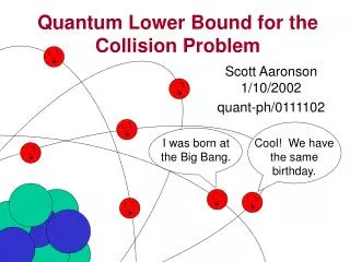
Quantum Lower Bound for the Collision Problem. I was born at the Big Bang. Cool! We have the same birthday. Scott Aaronson 1/10/2002 quant-ph/0111102. Collision Problem. Given . Promised: (1) X is one-to-one (permutation) or (2) X is two-to-one.

Quantum Lower Bound for the Collision Problem
E N D
Presentation Transcript
Quantum Lower Bound for the Collision Problem I was born at the Big Bang. Cool! We have the same birthday. Scott Aaronson 1/10/2002 quant-ph/0111102
Collision Problem • Given • Promised: • (1) X is one-to-one (permutation) or • (2) X is two-to-one • Problem: Decide which w.h.p., using few queries to the xi • Randomized alg: (n)
One-to-One Two-to-One
Result • Any quantum algorithm for the collision problem uses (n1/5) queries • Shi improved to (n1/4) • (n1/3) when |range| >> n • Previously no lower bound better than (1)
Implications • No polytime blackbox algorithms for • graph isomorphism • nonabelian hidden subgroup • breaking cryptographic hash functions
Implications 2. “Dynamical quantum theories” can’t be simulated in BQP, relative to oracle Define joint distribution over values of observable at times t1, t2, etc. (I.e. classical history) Given polytime quantum algorithm and set of “sampling points,” how hard to sample from this distribution?
Prepare and observe 2nd register • If X is 2-1, obtain (|i+|j)/2 with xi=xj How to Find a Collision in O(1) Queries If Your Memory Is Perfect • Sample 3. Hadamard every bit, and sample again 4. Hadamard every bit again (returning to (|i+|j)/2), and sample again Which basis state (|i or |j) were you “in” after Step 2? After Step 4?
Implications 3. |x|f(x) oracles (Kashefi et al. 2001) more powerful than |x|x|f(x) Requires (n1/7) lower bound for set comparison problem: given sequences x1…xn and y1…yn, decide whether {x1,…,xn}={y1,…,yn} or |{x1,…,xn,y1,…,yn}|>1.1n Can improve to (n1/6) using ideas of Shi
By end: Quantum Query Model • State after t queries: : workbits i: index to query z: output • Query: |,i,z |xi,i,z • Arbitrary unitaries that don’t depend on X
Brassard-Høyer-Tapp (1998) (n1/3) quantum alg for collision problem Grover’s algorithm over n2/3 xi’s Do I collide with any of the pink xi’s? n1/3 xi’s, queried classically, sorted for fast lookup
Lower Bound: Main Ideas • P(X)[0,1], even for g-1 inputs X with g>2. Surprisingly strong constraint. • Take uniform dist. over g-1 inputs • P becomes poly in g of deg 2T. Algebraic magic! • Use approximation theory to show T large
Proof: Let t,X,,i,z = amplitude of |,i,z after t queries. t,X,,i,z is poly of degt, by induction. Base case (t=0) trivial. Unitaries can’t increase degree. Query replaces t,X,,i,z by Lemma (follows Beals et al. 1998): Let (xi,h)=1 if xi=h, 0 otherwise. Then P(X) is poly of deg 2T over the (xi,h).
Let Input Distribution • D(g): Uniform distribution over g-1 inputs • Technicality: g might not divide n • But assume for simplicity that it does
Let • Then for some I, Monomials of P(X) • Claim: If T=O(n) then P(g) is a polynomial of degree 2T in g for integers 1gn. • I(X) = product of r variables (xi,h)
So • since Calculating (I,g): #1 • “Range” of I: Y. w=|Y|. • (I,g) = 0 unless YS (“range” of X)
# of g-1 inputs X with range S s.t. I(X)=1: Calculating (I,g): #2 • Given an S containing Y, # of g-1 inputs of size n: n!/(g!)n/g • Let {y1,…,yw} be distinct values in Y • ri = # of times yi appears in Y • r1 + … + rw = r
Polynomial in g of degree w + (r-w) = r 2T Becomes ~polynomial(g)
Markov’s Inequality Let P(x) be a poly with b1P(x)b2 for all a1xa2 and |dP(x*)/dx|c for some a1x*a2. Then Large derivative Short Long
Lower Bound • 0 P(g) 1 for all 0 g n • P(1) 1/10 and P(2) 9/10 • So dP/dg 4/5 somewhere • (n1/4) lower bound would follow if g always divided n
Acceptance prob. close to bivariate polynomial in g,N for all g|N s.t. How to Handle n mod g 0: Sketch • Choose N slightly larger than n such that g divides N • Choose g-1 function on {1,…,N} u.a.r, then subfunction of size n
Lower bound obtained when G=n2/5: (continued) • Restrict g’s range to [1,G]; then (g,N) points with g|N are plentiful, so P is bounded • P has large derivative somewhere in either the g or N directions
Large derivative between 1-1 and 2-1 Lots of points at which g|N so P is bounded
Shi’s Improvement to (n1/4) • Choose Nn s.t. g divides N, instead of Nn • If basis state | queries an undefined xi, | “drops out of the universe” • Result: Final state vector has norm in [0,1] Still OK! • P(g,N) is exactly polynomial in (g,N); so g’s range need not be restricted to [1,n2/5]
Uses Paturi’s inequality: • if 0p(x)1 for 0xn and p’()=(1) Shi’s Improvement to (n1/3) • For functions with range {1,…,3n/2}

