Efficient Algorithms for Sorting and Dynamic Sets Management
This text delves into advanced sorting algorithms and dynamic data structures, covering the complexities of sorting techniques like Radix Sort and Distribution Counting. It explores the efficiency of these algorithms, demonstrating how they outperform traditional methods in specific scenarios. Additionally, it discusses dynamic sets, including operations like insertion, deletion, and finding minimum or maximum elements. The focus is on leveraging data structures such as heaps and priority queues to optimize performance. Key concepts are presented throughout, including time complexity analyses and practical applications.

Efficient Algorithms for Sorting and Dynamic Sets Management
E N D
Presentation Transcript
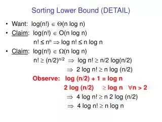
Sorting Lower Bound (DETAIL) • Want: log(n!) ÎQ(n log n) • Claim: log(n!) Î O(n log n) n! £ nnÞ log n! £ n log n • Claim: log(n!) ÎW(n log n) n! ³ (n/2)n/2Þ log n! ³ n/2 log(n/2) • Þ 2 log n! ³ n log (n/2) • Observe: log (n/2) + 1 = log n • 2 log (n/2) ³ log n "n > 2 • Þ 4 log n! ³ n 2 log (n/2) • Þ 4 log n! ³ n log n
Distribution Counting (8.2) • Array A contains n elements from {1,...,m}, m<<n for j = 0 to m-1 do count[j] = 0 // initialize m counters for i = 1 to n do // count incidences of each value count[A[i]] = count[A[i]] +1 for j = 1 to m-1 do // change to running totals of counts count[j] = count[j-1] + count [j] for i = n down to 1 do // put each type into auxiliary array B B[count[A[i]]] = A[i]; count [a[i]] = count[a[i]] - 1 for i =1 to n do A[i] = B[i] // copy back into original array • Complexity: O(n)
Radix Sort (A Linear-Time Sort) (8.3) • Suppose all n elements in sorting instance have bounded size, e.g., in {0, ..., rd –1} • Radix Sort • Make sure list is sorted with respect to each digit position, starting with rightmost digit position • Use distribution counting to sort at each digit position • Total of nd digit comparisons to sort n d-digit numbers 100 100 100 000 001 010 000 001 010 000 001 010 111 001 101 100 101 111 010 101 000 101 111 111
Dynamic Sets (III / Chapter 10) • Dynamic sets (data structures): • change a dictionary, e.g., add/remove words • reuse of structured information • fast updating for on-line algorithms • Elements: • key field is the element ID • dynamic set of key values • satellite information is not used in data organization • Operations • query: return information about the set • modify: change the set record x key satellite data
Dynamic Set Operations • Search(S,k) • Given set S and key value k, return pointer x to an element of S such that key[x] = k, or NIL if no such element query • Insert(S,x) • Augment set S with element pointed to by x modify • Delete(S,x) • Given pointer x to an element in set S, remove x from S modify • Minimum(S) / Maximum(S) • Given totally ordered set S, return pointer to element of S with smallest / largest key query
Dynamic Set Operations • Predecessor / Successor(S, x) • Given element x whose key is from a totally ordered set S, return a pointer to next smaller / larger element in S, or NIL if x is minimum / maximum element query • Union(S, S’) • Given two sets S, S’, return a new set S = S S’ modify
15 6 2 9 Elementary Data Structures (10.1/11.1 ) • Different data structures support/optimize different operations • Stack has top, LIFO policy • insert = push x: top(S) = top(S)+1); S[top(S)] = xO(1) • delete = pop O(1) • Queue has head, tail, FIFO policy • insert = enqueue: add element to the tail O(1) • delete = dequeue: remove element from the head O(1) 1 2 3 4 5 6 7 1 2 3 4 5 6 7 15 6 2 9 17 top[S] = 4 After push(S,17) top[S] = 5 1 2 3 4 5 6 7 1 2 3 4 5 6 7 15 6 2 9 15 6 2 9 8 head = 2 tail = 6 head = 2 After enqueue(Q,8) tail = 7 Note: head index is lower than tail index opposite of Figure 10.2 in textbook.
Priority Queue Abstract Data Structure (6.5) • Operations: • Insert(S,x): add element x • Minimum(S) / Maximum(S): return element with min/max key • DeleteMin(S) / DeleteMax(S): return min/max key, remove element • Applications • Simulation systems: key º event time • OS scheduler: key º job priority • Numerical methods key º inherent error in operation • Dijkstra’s shortest-path alg, Prim’s minimum spanning tree alg • Q: How do we use a PQ to sort? • A: Insert elements one by one; perform DeleteMin n times
What Are Naïve PQ Implementations? • Unordered list • Insert O(1) • DeleteMin O(n) • Ordered list • Insert O(n) • DeleteMin O(1) • If Insert, DeleteMin each accomplished in O(log n) time ÞO(n log n) sorting algorithm!
Heaps (6.1) • A heap is a binary tree of depth d such that • (1) all nodes not at depth d-1 or d are internal nodes each level is filled before the next level is started • (2) at depth d-1 the internal nodes are to the left of the leaves and have degree 2, except perhaps for the rightmost, which has a left child each level is filled left to right • A max heap (min heap) is a heap with node labels from an ordered set, such that the label at any internal node is ³ (£) the label of any of its children All root-leaf paths are monotone
Heaps, and Sorting With Heaps • (Every node in a heap is the root of a heap!) • How do we store a heap? • Implicit data structure: // maxheap example Array index: 1 2 3 4 5 6 7 8 9 10 Value: 20 11 5 5 3 2 3 4 1 2 • A[i] is parent of A[2i] and A[2i+1] • How do we sort using a heap? • Insert: Put new value at A[n]; fix violation of heap condition (“re-heapify”) • DeleteM*: Remove root; replace by A[n]; re-heapify • If maxheap, DeleteMax (return largest element first) • If minheap, DeleteMin (return smallest element first)
Heaps (6.1/7.1) • Pointers: • Parent parent of A[i] has index = i div 2 • Left, Right (children) children of A[i] have indices 2i, 2i+1 • Parent Child this is a minheap example 2 1 1 2 3 4 5 6 7 8 9 10 6 4 2 6 4 8 11 5 9 10 13 12 2 3 8 11 5 9 4 5 6 7 10 13 12 8 9 10
Heap Operations (6.2-5/7.2-5) Insert(S,x): O(height) O(log n) 2 2 2 4 6 4 6 6 3 8 11 7 9 8 3 7 9 8 7 9 4 11 3 11 10 13 12 10 13 12 10 13 12 Keep swapping with parent until heap condition satisfied 2 12 4 4 6 4 6 4 6 12 6 5 8 11 5 9 8 11 5 9 8 11 5 9 8 11 12 9 10 13 12 10 13 10 13 10 13 Extract-min(S): return head, replace head key with the last key, float down O(log n) “Float down”: If heap condition violated, swap with smaller child
Heapsort (6.4/7.4) • Build heap: n x O(log n) time • for i= 1..n do insert (A[1..i],A[i]) • Extract elements in sorted order: n x O(log n) time • fori = n..2 do • Swap (A[1] A[i]) • Heapsize = Heapsize-1 • Float down A[1] 4 12 5 13 6 5 6 5 6 6 7 7 8 11 7 9 8 11 7 9 12 12 8 11 9 8 11 9 10 13 12 10 13 4 5 10 13 4 10 4 13 6 7 13 12 11 7 7 8 8 9 8 10 12 12 10 11 9 10 11 9 13 9 8 7 12 10 11 5 4 6 5 5 4 4 13 6 5 4 6
Actual Time To Build Heap = O(n) (6.3) • Heapify (i,j) makes range [i,j] satisfy heap property: Heapify (i,j) // minheap example if i not a leaf and child of i is > i let k = larger child of i interchange a[i], a[k] Heapify (k,j) • BuildHeap: for i=n to 1 do Heapify (i,n) • Observe: If vertices i+1, ..., n are roots of heaps, then after Heapify(i,n) vertices i,...,n will be roots of heaps • Let T(h) º time for Heapify on v at height h T(h)= O(h) • Heapify called once for each v Þ total BuildHeap time is O(Svh(v)) • Vertex at height i is root of heap with 2i+1 nodes Þén/2i+1ù vertices at height i • S i×n/2i is upper bound on BuildHeap time (S i/2i = 2 O(n))
Divide and Conquer • First “paradigm” or “framework” DQ(S) if S is small return ADHOC(S) else decompose S into subproblems S1 ,…, Sk // divide for i = 1 to k do yi = DQ(Si ) // conquer recombine yi into solution y // compose return y • “Universal method”: Mergesort, Quicksort, FFT, Matrix/Integer arithmetic are classic examples
DQ for the MaxMin Problem • Remember from first lecture: Given list of n numbers, return largest and smallest • Naïve: 2(n-1) or 2n-1 comparisons (two passes) • DQ approach n = 1 0 comparisons needed n = 2 1 comparison needed else: bisect list make recursive calls return max(max1, max2), min(min1, min2) • #comparisons: T(n) = T(ën/2û) + T(én/2ù) + 2, n > 2
DQ for the MaxMin Problem • T(n) = T(ën/2û) + T(én/2ù) + 2, n > 2 • Transform with S(k) = T(2k) S(k) = 2S(k-1) + 2 Note: The recurrence a0tn + a1t n-1 + … + akt n-k = bn p(n) has solution tn = Si=1,kcirin where ri are roots of the C.P.: (a0xk + a1x k-1 + … + ak) (x – b)d+1 = 0 S(n) – 2S(n-1) = 1n× 2 Þa0 = 1, a1 = -2, b = 1, p(n) = 2, d = 0 ÞC.P. = (x-2)(x-1)1 ÞS(k) = c12k + c21k • Initial conditions: S(1) = c1×2 + c2 = 1 ; S(2) = c1×4 + c2 = 4 Þc1 = 3/2, c2 = -2 • T(n) = T(2k ) = S(k) = 3/2 × 2log2n – 2 = 3n/2 – 2
Intuitive MaxMin Lower Bound • “Information argument” • Start: Nothing known about n elements • End: “Neither Max nor Min” known about all but 2 elements • Four “buckets” • Know Nothing • Not Max • Not Min • Neither Max nor Min Know Nothing Not Max Not Min Neither Max nor Min n/2 - 1 n/2 n/2 - 1
Divide and Conquer for Sorting (2.3/1.3) • Divide (into two equal parts) • Conquer (solve for each part separately) • Combine separate solutions • Mergesort • Divide into two equal parts • Sort each part using Mergesort (recursion!!!) • Merge two sorted subsequences
Merging Two Subsequences x[1]-x[2]- … - x[k] y[1]-y[2]- … - y[l] if y[i] > x[j] y[i+1] > x[j] < k+l-1 edges = # (comparisons) = linear time
179 310 351 652 285 179 179 310 310 351 351 652 652 423 423 423 861 861 861 254 254 254 450 450 450 520 520 520 179 179 310 285 285 285 310 179 310 351 652 351 652 351 423 423 423 423 423 450 861 861 861 861 520 254 254 254 254 652 450 450 450 450 861 520 520 520 520 179 179 179 254 285 285 310 310 310 351 351 351 652 652 652 423 423 423 861 861 861 254 254 254 450 450 450 520 520 520 179 285 285 285 310 351 652 285 254 450 520 423 861 254 450 520 254 450 520 310 179 179 652 652 351 351 423 423 423 861 861 861 254 450 520 179 285 310 179 351 652 351 652 423 861 285 179 652 351 423 254 861 423 450 520 861 254 285 285 254 450 520 310 285 310 310 450 520 285 285 310 310 285 423 861 254 285 310 310 179 351 652 179 179 179 351 652 652 351 351 450 520 652 Merge Sort Execution Example
1 2 3 4 5 6 7 8 1 3 5 8 2 4 6 7 1 5 3 8 4 7 2 6 5 1 5 1 7 4 6 2 Recursion Tree log n • n comparisons per level • log n levels • total runtime = n log n
Quicksort (7.1-7.2/8.1-8.2) • Sorts in placelike insertion sort, unlike merge sort • Divideinto two parts such that • elements of left part < elements of right part • Conquer: recursively solve for each part separately • Combine: trivial - do not do anything • Quicksort(A,p,r) • if p <r • then q Partition(A,p,r) • Quicksort(A,p,q) • Quicksort(A,q+1,r) //divide //conquer left //conquer right
Divide = Partition PARTITION(A,p,r) //Partition array from A[p] to A[r] with pivot A[p] //Result: All elements original A[p] has index i x = A[p] i = p - 1 j = r + 1 repeat forever repeat j = j - 1 until A[j] x repeat i = i +1 until A[i] x if i < j then exchange A[i] A[j] else return j
9 9 7 7 6 6 15 15 16 16 5 5 10 10 11 11 i i j j 9 7 6 15 16 5 10 11 5 7 6 15 16 9 10 11 9 7 6 15 16 5 10 11 left left left left left right right right right right i i j 5* 7 6 15 16 j 9* 10 11 9 7 6 15 16 5 10 11 i 5 7 6 15 16 9 10 j 11 9 7 6 15 16 5 10 11 5 5 5 7 7 7 6 6 6 15 15 15 16 16 16 9 9 9 10 10 10 11 11 11 5 5 7 7 6 6 15 15 16 16 9 9 10 10 11 11 5 7 6 15 16 9 10 11 5 5 5 i 7 7 7 6 6 6 15 15 15 16 16 16 9 9 9 10 10 10 11 11 11 j i left right j i i j j i i 5 7 6 j j 15 16 j 9 10 11 left right i i 5 5 5 5 5 9 5 7 7 7 7 7 7 7 6 6 6 6 6 6 6 15 15 15 15 15 15 15 j 16 16 16 16 16 16 16 9 9 9 5 9 9 9 j 10 10 10 10 10 10 10 11 11 11 11 11 11 11 j i i i left j j j right 9 7 6 15 16 5 10 11 left right 9 9 left 7 7 6 6 15 15 16 16 5 5 right 10 10 11 11 i j left left right right i i j i j left right i i j left right 5 7 6 15 16 9 10 11 i i left right left right j j left left left right right right left right 5 6 7 15 16 9 10 11 5 6 7 11* 16 9 10 15* 5 left left 7 6 15 16 right right 9 10 11 5 6 7 11 10 9 16 15 j j 5 5 7 6 6 7 15 15 16 16 9 9 10 10 11 11 i j 5 6 7 11 10 9 16 15 left right 5 6 7 15 16 9 10 11 i 5 j 7 6 15 16 9 10 11 5 6 7 11 10 9 16 15 5 5 5 7 6 6 6 7 7 15 9 11 16 10 16 9 11 9 10 15 10 11 16 15 i 5 5 6 6 7 7 j 9 9 10 10 11 11 16 15 15 16 j i i j i j 5 5 6 6 7 7 15 11 16 16 9 9 10 10 15 11 i j j i j 5 6 7 15 16 9 10 11 i i j j i How It Works
0123456789 0 123456789 n 89 8 9 Runtime of Quicksort • Worst case: • every time nothing to move • pivot = left (right) end of subarray • O(n2)
Runtime of Quicksort • Best case: • every time partition in (almost) equal parts • no worse than in given proportion • O(n log n) • Average case • O(n log n) ??? • How do we prove this?
Master Method (4. 3) Recurrent formulaT(n) = aT(n/b) + f(n) 1) If for some > 0 then 2) If then 3) If for some > 0 and a f(n/b) c f(n) for some c < 1 then
Master Method Examples • Mergesort T(n) = 2T(n/2) + (n) • Strassen (28.2) T(n) = 7T(n/2) + (n^2)