Introduction to Probability: Concepts and Distributions of Random Variables
This unit covers essential concepts of probability, including definitions of random variables, population, and events. You will learn about the probability of events, their frequencies, and how to estimate them through random sampling. The unit highlights discrete (binomial) and continuous (normal) distributions, emphasizing their characteristics and applications. We also explore binomial random variables, their parameters, and provide examples, including calculations for determining probabilities and cumulative probabilities.


Introduction to Probability: Concepts and Distributions of Random Variables
E N D
Presentation Transcript
4: Probability Part A: Concepts & binomial distributions Part B: Normal distributions Unit 4: Intro to probability
Definitions • Random variable a numerical quantity that takes on different values depending on chance • Population the set of all possible values for a random variable • Event an outcome or set of outcomes for a random variable • Probability the proportion of times an event occurs in the population; (long-run) expected proportion Unit 4: Intro to probability
Probability (definition #1) The probability of an event is its relative frequency (proportion) in the population. Example: Let A selecting a female at random from an HIV+ population There are 600 people in the population. There are 159 females. Therefore, Pr(A) = 159 ÷ 600 = 0.265 Unit 4: Intro to probability
Probability (definition #2) The probability of an event is its expected proportion when the process in repeated again and again under the same conditions • Select 100 individuals at random • 24 are female • Pr(A) 24 ÷ 100 = 0.24 • This is only an estimate (unless n is very very big) Unit 4: Intro to probability
Probability (definition #3) The probability of an event is a quantifiable level of belief between 0 and 1 Example: Prior experience suggests a quarter of population is female. Therefore, Pr(A) ≈ 0.25 Unit 4: Intro to probability
Some rules of probability Unit 4: Intro to probability
Types of random variables • Discrete have a finite set of possible outcomes, • e.g. number of females in a sample of size n (0, 1, 2, …, n) • We cover binomial random variables • Continuous have a continuum of possible outcomes • e.g., average body weight (lbs) in a sample (160, 160.5, 160.75, 160.825, …) • We cover Normal random variables There are other random variable families, but only binomial and Normal RVs are covered for now. Unit 4: Intro to probability
Binomial distributions • Most popular type of discrete RV • Based on Bernoulli trial random event characterized by “success” or “failure” • Examples • Coin flip (heads or tails) • Survival (yes or no) Unit 4: Intro to probability
Binomial random variables • Binomial random variable random number of successes in n independent Bernoulli trials • A family of distributions identified by two parameters • n number of trials • p probability of success for each trial • Notation: X~b(n,p) • X random variable • ~ “distributed as” • b(n, p) binomial RV with parameters n and p Unit 4: Intro to probability
“Four patients” example • A treatment is successful 75% of time • We treat 4 patients • X random number of successes, which varies 0, 1, 2, 3, or 4 depending on binomial distribution X~b(4, 0.75) Unit 4: Intro to probability
The probability of i successes is … Binomial formula Where nCi= the binomial coefficient (next slide) p = probability of success for each trial q = probability of failure =1 – p Unit 4: Intro to probability
Binomial coefficient (“choose function”) where ! the factorial function: x! = x (x – 1) (x – 2) … 1 Example: 4! = 4 3 2 1 = 24 By definition 1! = 1 and 0! = 1 nCi the number of ways to choose i items out of n Example: “4 choose 2”: Unit 4: Intro to probability
“Four patients” example • n = 4 and p = 0.75 (so q = 1 - 0.75 = 0.25) • Question: What is probability of 0 successes? i = 0 • Pr(X = 0) =nCi pi qn–i = 4C0 · 0.750 · 0.254–0= 1 · 1 · 0.0039 = 0.0039 Unit 4: Intro to probability
X~b(4,0.75), continued Pr(X = 1) = 4C1· 0.751 · 0.254–1 = 4 · 0.75 · 0.0156 = 0.0469 Pr(X = 2) = 4C2· 0.752 · 0.254–2 = 6 · 0.5625 · 0.0625 = 0.2106 (Do not demonstrate all calculations. Students should prove to themselves they derive and interpret these values.) Unit 4: Intro to probability
X~b(4, 0.75) continued Pr(X = 3) = 4C3· 0.753 · 0.254–3 = 4 · 0.4219 · 0.25 = 0.4219 Pr(X = 4) = 4C4· 0.754 · 0.254–4 = 1 · 0.3164 · 1 = 0.3164 Unit 4: Intro to probability
The distribution X~b(4, 0.75) Probability table for X~b(4,.75) Probability curve for X~b(4,.75) Unit 4: Intro to probability
Get it? Pr(X = 2) = .2109 Area under the curve (AUC) concept The area under a probability curve (AUC) = probability! Unit 4: Intro to probability
Cumulative probability (left tail) • Cumulative probability = Pr(X i) = probability less than or equal to i • Illustrative example: X~b(4, .75) • Pr(X 0) = Pr(X = 0) = .0039 • Pr(X 1) = Pr(X 0) + Pr(X = 1) = .0039 + .0469 = 0.0508 • Pr(X 2) = Pr(X 1) + Pr(X = 2) = .0508 + .2109 = 0.2617 • Pr(X 3) = Pr(X 2) + Pr(X = 3) = .2617 + .4219 = 0.6836 • Pr(X 4) = Pr(X 3) + Pr(X = 4) = .6836 + .3164 = 1.0000 Unit 4: Intro to probability
X~b(4, 0.75) Unit 4: Intro to probability
Bring it on! Cumulative probability left tail = cumulative probability Area under shaded bars in left tail sums to 0.2617, i.e., Pr(X 2) = 0.2617 Area under “curve” = probability Unit 4: Intro to probability
Reasoning Use probability model to reasoning about chance. I hypothesize p = 0.75, but observe only 2 successes. Should I doubt my hypothesis? ANS: No. When p = 0.75, you’ll see 2 or fewer successes 25% of the time (not that unusual). Unit 4: Intro to probability
StaTable probability calculator • Link on course homepage • Three versions • Java (browser) • Windows • Palm Probability Cumulative probability Unit 4: Intro to probability
Intro to Probability, Part B The Normal distributions Unit 4: Intro to probability
How’s my hair? Looks good. The Normal distributions • Most popular continuous model • Recognized by de Moivre (1667– 1754) • Extended by Laplace (1749 – 1827) Unit 4: Intro to probability
Probability density function (curve) • Example: vocabulary scores of 947 seventh graders • Smooth curve drawn over histogram is a model of the actual distribution • Mathematical model is the Normal probability density function (pdf) Unit 4: Intro to probability
Area under curve • The area under the curve (AUC) concepts applies • The shaded bars (left tail) represent scores ≤ 6.0 = 30.3% of scores • Pr(X ≤ 6) = 0.303 Unit 4: Intro to probability
Areas under curve (cont.) • Now translate this to the area under the curve (AUC) • The scale of the Y-axis is adjusted so the total AUC = 1 • The AUC to the left of 6.0 (shaded) = 0.293 • Therefore, the AUC “models” the area in proportion area in the bars of the histogram, i.e., probabilities of associated ranges Unit 4: Intro to probability
Density Curves Unit 4: Intro to probability
Normal distributions • Normal distributions = a family of distributions with common characteristics • Normal distributions have two parameters • Mean µ locates center of the curve • Standard deviation quantifies spread (at points of inflection) Arrows indicate points of inflection Unit 4: Intro to probability
68-95-99.7 rule for Normal RVs • 68% of AUC falls within 1 standard deviation of the mean (µ) • 95% fall within 2 (µ2) • 99.7% fall within 3 (µ 3) Unit 4: Intro to probability
Illustrative example: WAIS Wechsler adult intelligence scores (WAIS) vary according to a Normal distribution with μ = 100 and σ = 15 Unit 4: Intro to probability
Another example (male height) • Adult male height is approximately Normal with µ = 70.0 inches and = 2.8 inches (NHANES, 1980) • Shorthand: X ~ N(70, 2.8) • Therefore: • 68% of heights = µ = 70.0 2.8 = 67.2 to 72.8 • 95% of heights = µ 2 = 70.0 2(2.8) = 64.4 to 75.6 • 99.7% of heights = µ 3 = 70.0 3(2.8) = 61.6 to 78.4 Unit 4: Intro to probability
68% (by 68-95-99.7 Rule) ? 16% 16% -1 +1 70 72.8 (height) 84% Another example (male height) What proportion of men are less than 72.8 inches tall? (Note: 72.8 is one σ above μ) Unit 4: Intro to probability
? 68 70 (height) Male Height Example What proportion of men are less than 68 inches tall? 68 does not fall on a ±σ marker. To determine the AUC, we must first standardize the value. Unit 4: Intro to probability
Standardized value = z score To standardize a value, simply subtract μ and divide by σ This is now a z-score The z-score tells you the number of standard deviations the value falls from μ Unit 4: Intro to probability
Example: Standardize a male height of 68” Recall X ~ N(70,2.8) Therefore, the value 68 is 0.71 standard deviations below the mean of the distribution Unit 4: Intro to probability
? 68 70 (height values) Men’s Height (NHANES, 1980) What proportion of men are less than 68 inches tall? = What proportion of a Standard z curve is less than –0.71? -0.71 0 (standardized values) You can now look up the AUC in a Standard Normal “Z” table. Unit 4: Intro to probability
Using the Standard Normal table Pr(Z≤ −0.71) = .2389 Unit 4: Intro to probability
.2389 68 70 (height values) -0.71 0 (standardized values) Summary (finding Normal probabilities) • Draw curve w/ landmarks • Shade area • Standardize value(s) • Use Z table to find appropriate AUC Unit 4: Intro to probability
68 70 (height values) -0.71 0 (standardized values) Right-”tail” • What proportion of men are greater than 68” tall? • Greater than look at right “tail” • Area in right tail = 1 – (area in left tail) .2389 1- .2389 = .7611 Therefore, 76.11% of men are greater than 68 inches tall. Unit 4: Intro to probability
Z percentiles • zp the z score with cumulative probability p • What is the 50th percentile on Z? ANS: z.5 = 0 • What is the 2.5th percentile on Z? ANS: z.025 = 2 • What is the 97.5th percentile on Z? ANS: z.975 = 2 Unit 4: Intro to probability
Finding Z percentile in the table • Look up the closest entry in the table • Find corresponding z score • e.g., What is the 1st percentile on Z? • z.01 = -2.33 • closest cumulative proportion is .0099 Unit 4: Intro to probability
.10 ? 70 (height values) Unstandardizing a value How tall must a man be to place in the lower 10% for men aged 18 to 24? Unit 4: Intro to probability
Table A:Standard Normal Table • Use Table A • Look up the closest proportion in the table • Find corresponding standardized score • Solve for X (“un-standardize score”) Unit 4: Intro to probability
Table A:Standard Normal Proportion .08 1.2 .1003 Pr(Z < -1.28) = .1003 Unit 4: Intro to probability
.10 ? 70 (height values) Men’s Height Example (NHANES, 1980) • How tall must a man be to place in the lower 10% for men aged 18 to 24? -1.28 0 (standardized values) Unit 4: Intro to probability
Observed Value for a Standardized Score • “Unstandardize” z-score to find associated x : Unit 4: Intro to probability
Observed Value for a Standardized Score • x = μ + zσ = 70 + (-1.28 )(2.8) = 70 + (3.58) = 66.42 • A man would have to be approximately 66.42 inches tall or less to place in the lower 10% of the population Unit 4: Intro to probability