Download
1 / 28
300 likes | 550 Vues
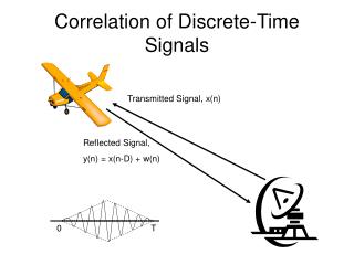
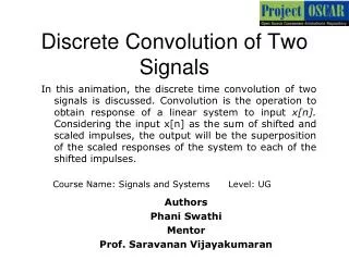
This animation explores the concept of discrete convolution, a key operation used to determine the response of linear systems to discrete-time input signals, denoted as x[n]. By treating the input as a sum of shifted and scaled impulses, the output represents the superposition of scaled responses of the system to these impulses. The learning objectives include explaining convolution and performing calculations involving discrete signals. This interactive content is designed for undergraduate students in a Signals and Systems course.

E N D
Discrete Convolution of Two Signals In this animation, the discrete time convolution of two signals is discussed. Convolution is the operation to obtain response of a linear system to input x[n]. Considering the input x[n] as the sum of shifted and scaled impulses, the output will be the superposition of the scaled responses of the system to each of the shifted impulses. Course Name: Signals and Systems Level: UG Authors Phani Swathi Mentor Prof. Saravanan Vijayakumaran
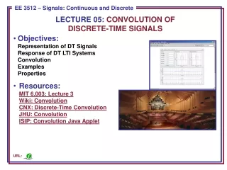
Learning Objectives After interacting with this Learning Object, the learner will be able to: • Explain the convolution of two discrete time signals
Definitions of the components/Keywords: 1 • Convolution of two signals: • The x[n] and h[n] are the two discrete signals to be convolved. • The convolution of two signals is denoted by • which means • where k is a dummy variable. 2 3 4 5
Master Layout (Part 1) This animation consists of 2 parts: Part 1 – First method of convolution – Method 1 Part 2 – Alternate method of convolution – Method 2 1 Lines and dots have to appear at the same time. This is applicable to all figures Signals taken to convolve Shifted version of h[n] Scaled version of h[n] 2 3 4 5
Step 1: 1 2 3 4 5
Step 2: Overall calculation of y[n] 1 X[1]h[n-1] 3 2 1 2 0 1 2 3 n X[2]h[n-2] h[n-2] 6 4 2 3 2 1 3 0 1 2 3 4 n 0 1 2 3 4 n h[n-3] 3 2 1 X[3]h[n-3] 3 2 1 4 0 1 2 3 4 5 n 0 1 2 3 4 5 n 5
Step 3: 1 X[1]h[n-1] x[1]h[n-1] 3 2 1 2 0 1 2 3 n 3 4 5
Step 4: Step 1 1 X[2]h[n-2] 6 5 4 3 2 1 h[n-2] X[2] h[n-2] 3 2 1 2 2 3 0 1 2 3 4 n 0 1 2 3 4 n 4 4 5 5
Step 5: 1 X[3]h[n-3] h[n-3] x[3]h[n-3] 3 2 1 3 2 1 2 3 0 1 2 3 4 5 n 0 1 2 3 4 5 n 4 5
Step 6: Y[n] 1 1 8 7 6 5 4 3 2 1 Y[n] 2 2 3 0 1 2 3 4 5 6 7 8 n 4 4 5 5
Electrical Engineering Use STAM template Slide 1 Slide 3 Slide 26 Slide 28 Slide 27 Introduction Definitions Analogy Test your understanding (questionnaire) Lets Sum up (summary) Want to know more… (Further Reading) Interactivity: The correct answer is shown in red Try it yourself Fig. A Fig. B Fig. C Fig. 1 Fig. 2 Demo Activity Fig. A Fig. C Fig. B 11 Instructions/ Working area Credits
Interactivity option 1: Step No 1: 1 y[n] h[n] x[n] 3 2 1 3 2 1 3 2 1 2 0 1 2 3 4 5 0 1 2 3 4 5 3 Fig. 1 Fig. 2 0 1 2 3 4 5 n -1 0 1 2 3 4 5 n Fig.1 Fig.2 4 5
Interactivity option 1: Step No 2: 1 y[n] Y[n] Y[n] 12 10 8 6 4 2 12 10 8 6 4 2 3 2 1 2 0 1 2 3 4 5 0 1 2 3 4 5 3 Fig. 1 Fig. 2 0 1 2 3 4 5 6 n 0 1 2 3 4 5 6 n a) Fig. A b) Fig. B 4 5
Interactivity option 1: Step No 3: 1 y[n] Y[n] 12 10 8 6 4 2 3 2 1 2 0 1 2 3 4 5 0 1 2 3 4 5 3 Fig. 1 Fig. 2 0 1 2 3 4 5 6 n c) Fig. C 4 5
Master Layout (Part 2) 1 This animation consists of 2 parts: Part 1 – First method of Convolution – Method 1 Part 2 – Alternate method of Convolution – Method 2 Signals taken to convolve h[n] X[n] 2 1 2 3 ……. -3 -2 -1 0 1 2 3 ……. 3 Result signal of convolution The dotted lines represent y[n] The thicker line represents only y[4] 4 5
Step 1: 1 X[n] h[n] 2 2 1 2 3 n 3 ….-3 -2 -1 0 1 2 3….. 4 5
Step 2: 1 h[n-k] X[k] 3 2 2 1 2 k=n-2 k=n-1 k= n k 3 -3 -2 -1 0 1 2 3 4 5
Step 3: 1 2 3 4 5
Step 4: 1 X[k] h[4-k] 2 2 3 4 k 3 -3 -2 -1 0 1 2 3 4 5
Step 5: 1 X[k]h[4-k] X[k]h[4-k] 6 4 2 2 2 3 4 3 4 5
Step 6: Y[4] 1 1 12 10 8 6 4 2 Y[4] 2 2 3 0 1 2 3 4 5 6 7 8 9 n 4 4 5 5
Electrical Engineering Use STAM template Slide 1 Slide 3 Slide 26 Slide 28 Slide 27 Introduction Definitions Analogy Test your understanding (questionnaire) Lets Sum up (summary) Want to know more… (Further Reading) Interactivity: Try it yourself Fig. a Fig. b Fig. c Fig. 3 Fig. 4 Demo Activity Fig. a Fig. b Fig. c 22 Instructions/ Working area Credits
Interactivity option 1: Step No 1: 1 y[n] x[n] h[5-k] 3 2 1 3 2 1 4 3 2 1 2 0 1 2 3 4 5 0 1 2 3 4 5 3 Fig. 1 Fig. 2 0 1 2 3 4 5 6 n 0 1 2 3 4 5 6 n Fig.3 Fig.4 4 5
Interactivity option 1: Step No 2: 1 y[n] 4 3 2 1 3 2 1 3 2 1 Y[5] Y[5] 2 0 1 2 3 4 5 0 1 2 3 4 5 3 Fig. 1 Fig. 2 0 1 2 3 4 5 6 n 0 1 2 3 4 5 6 n a) Fig. a b) Fig. b 4 5
Interactivity option 1: Step No 3: 1 y[n] Y[5] 4 3 2 1 3 2 1 2 0 1 2 3 4 5 0 1 2 3 4 5 3 Fig. 1 Fig. 2 0 1 2 3 4 5 6 n c) Fig. c 4 5
Questionnaire 3 2 1 1 3 2 1 1. Find the value of y[6] Answers: a) b) 2.The Convolution sum is given as ___________ Answers: The correct answers are given in red. h[n] x[n] 2 0 1 2 3 4 5 6 0 1 2 3 4 5 6 10 8 6 4 2 8 6 4 2 3 4 0 1 2 3 4 5 6 0 1 2 3 4 5 6 5
Linksfor further reading Reference websites: Books: Signals & Systems – Alan V. Oppenheim, Alan S. Willsky, S. Hamid Nawab, PHI learning, Second edition. Research papers:
Summary • In discrete time, the representation of signals is taken to be the weighted sums of shifted unit impulses. • This representation is important, as it allows to compute the response of an LTI(Linear Time Invariant) system to an arbitrary input in terms of the system’s response to a unit impulse. • The convolution sum of two discrete signals is represented as where • The convolution sum provides a concise, mathematical way to express the output of an LTI system based on an arbitrary discrete-time input signal and the system‘s response.