Download
1 / 1
10 likes | 104 Vues
Background. Discrete time receivers are useful because they can be implemented in software defined radios, DSPs, and other digital hardware rather than in traditional analog or continuous time systems.

E N D
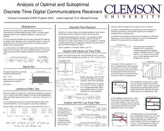
Background Discrete time receivers are useful because they can be implemented in software defined radios, DSPs, and other digital hardware rather than in traditional analog or continuous time systems. All of the examined systems use the same signal set and assume an additive white Gaussian noise channel with signal to noise ratio Eb/N0 where Eb is the bit energy and N0/2 is the power spectral density of the noise process. In continuous time, the ideal receiver uses a filter matched to the signal set. This results in the error probability shown. The discrete time receivers examined attempt to approach this performance level. Likelihood Ratio Test Detector design that utilizes the conditional probabilities of seeing a 0 or a 1 given a vector R of samples. The ratio of the probabilities is taken and tested against a threshold of 1 (choose s0 if less and s1 if greater). The log-likelihood ratio test is a variant that takes the logs of the ratio and threshold. Can be simpler to use in some situations. Define sample vector R and covariance matrix K (built from Rx()). System with Summer Receivers take N samples in T seconds. RC is chosen as a compromise between the optimal values for different values of N. Note that Rx() is a function of N0 and RC and b is the expected value of the sample vector for bit b. System with Discrete Time Correlator System with Ideal Low Pass Filter System uses ideal low pass filter with bandwidth (B) set to ensure that N uncorrelated samples are possible: t0 = T\N = 1\2B, B = N\2T System with Log-Likelihood Ratio Test Error Probability Ideal Continuous Time Receiver Two values of N are examined. For N=10, the samples are evenly spaced, centered at 0.5. For N=3, the sample are evenly spaced in the second half of the signal period. Note that there is much more power in the signal during the second half of the signal period. System assumption that the ideal LPF does not distort the signal is invalid for narrow filter bandwidth. Error probability does not depend on N, only A, T, and N0, therefore, for uncorrelated samples, taking extra samples does not improve probability of correct detection. Sample Times Error probability curves for N=10. Note that LLR is best, followed by Correlator and then Summer. Also, curves are widely spaced because samples taken early in sample period have relatively low signal power and are more affected by noise. Signal for Binary 0 Signal Set P(e) Curves for N=10 LLR Sensitivity to N0 P(e) Curves for N=3 All examined systems use binary antipodal signaling where: s0(t) = -s1(t) Basic waveform is a pulse with amplitude A and duration T: s0(t)=ApT(t) System Parameters Autocorrelation Function Filtered White Noise System Parameters Error probability curves for N=3. Note that curves are in the same order, but much closer together. This is due to the fact that the 3 samples all have relatively high signal power and thus are less affected by noise in the channel. Discrete Time Receiver System with RC Low Pass Filter Error Probability Calculation Objective is to take multiple uncorrelated samples of each symbol period and use them to determine which symbol was sent. A tradeoff exists between the number of uncorrelated samples possible and the bandwidth of the filter used. As the filter is narrowed, the noise autocorrelation function spreads out, resulting in fewer opportunities for independent samples. May be forced to take correlated samples as a result. Take N samples in T seconds, define t0 as T/N System uses a continuous-time RC low-pass filter and one of three discrete-time receivers. Objective is to compare relative performance of the three receivers. LLR dependence on N0 would require more complicated receiver, but not in this case. Changing N0 in this system only multiplies K matrix by a scalar, which does not affect LLR since a threshold of 0 is used. LLR only depends on ratios of elements of K, not actual magnitudes. System Block Diagram Analysis of Optimal and Suboptimal Discrete-Time Digital Communications Receivers Clemson University SURE Program 2005 Justin Ingersoll, Prof. Michael Pursley Summer: takes N samples and compares sum to threshold Correlator: multiplies R by its expected value and compares to a threshold, improving on the summer by giving more weight to samples with more signal power. LLR: performs log-likelihood ratio test and compares to a threshold, improving on the correlator by taking into account the relationship between the samples via the correlation matrix.