Download
1 / 43
430 likes | 647 Vues
TDDC47: Real-time and Concurrent Programming Lecture 8: Real-time communication. Simin Nadjm-Tehrani Real-time Systems Laboratory Department of Computer and Information Science Linköping university. Reading material. TDDD07: H. Kopetz 2003 article (see course web)

E N D
TDDC47: Real-time and Concurrent Programming Lecture 8: Real-time communication Simin Nadjm-Tehrani Real-time Systems Laboratory Department of Computer and Information ScienceLinköping university
Reading material TDDD07: • H. Kopetz 2003 article (see course web) • Davis et al 2007 article (- ” -) TDDC47: • Course compendium • Davis et al 2007 article (see course web)
From last lectures • In two scheduling lectures we looked at • Single processor hard real-time scheduling • TDDD07: • Distributed case with dynamic load • Time and clocks in distributed systems ...
Real-time communication • This lecture: How can the communication network and protocols support real-time? • RT communication is about scheduling the communication medium – NOT the CPU ...
Distributed applications • Assume that tasks are run on different nodes according to some local scheduling • Nodes need to exchange data • messages need to reach destination before their deadline ...
Real-time constraints • When message transmissions must have a well-defined time bound for the system to meet it deadlines • So called end-to-end deadlines • Example: shortly after each braking, brake light must know it in order to turn on!
Two approaches • We will look at two dominant methods for bus scheduling • Time triggered (TTP) • Event triggered (CAN) • Used extensively in automotive and aerospace applications
Node n-1 Time-triggered protocol (TTP) • Origin in research projects in Vienna in early 90´s [Kopetz et.al] • Time division multiple access (TDMA) … Node n Node 1
Node n-1 … Node n Node 1 … Communication protocol • Message Description List: allocates a pre-defined slot within which each node can send its (pre-defined) message A TDMA round
Message scheduling • TDMA round implemented through the MEDL (message description list) • MEDL has a static schedule for each message • No constraints on (local) node CPU scheduling
Temporal firewall Host Host Node n CNI … CC CC • CNI provides temporally accurate state information (via clock synchronisation) • When the data is temporally not valid, it can no longer be exchanged
Host Host CNI … CC CC BG BG BG BG BG BG BG BG BG Replication & failure detection BG: Buss Guardian (stops babbling idiots)
The major success of the TTP bus is due to the possibility of detecting arbitrary (Byzantine) failures • We will come back to this later…
Two approaches • We will look at two dominant methods for bus scheduling • Time triggered (TTP) • Event triggered (CAN) • Used extensively in automotive and aerospace applications
The CAN bus • Controller area network that exists in all cars built in Europe today • Compulsory for the on-board diagnostics in USA car models from 2008 • Why? • Imagine: 2500 signals, 32 ECUs on one bus Amount of wires…
Predecessor to CAN (1976) Ethernet: • Current versions give high bandwidth but time-wise nondeterministic • CSMA/CD • Sense before sending on the medium (Carrier Sense: CS) • All nodes broadcast to all (Multiple Access: MA) • If collision, back off and resend (Collision Detection: CD)
Collisions • Ethernet has high throughput but temporally nondeterministic Node 2 & 3 start to send Node 3 waits for sending Node 2 waits for sending Node 1 sends Collision
Backoff • The period for waiting after a collision • Each node waits up to two “slot times” after a collision (random wait) • If a new collision, the max. backoff interval is doubled • After 10 attempts the node stops doubling • After 16 attempts declares an error
Treating non-determinism How often? • Model the network throughput and compute probabilistic guarantees that collisions will not be too often • Theoretical study:With 100Mbps, sending 1000 messages of 128 bytes per second, there is a 99% probability that there will be a 1 ms delay over ~1140 years [www.rti.com Ethernet study] • Make collision resolution deterministic!
CAN protocol • Developed by Bosch and Intel (1986) • ISO Standard 1993 • Highest bandwidth 1Mbps, ~40-50m • CSMA/CR: broadcast to all nodes • CR: Collision resolution by bit-wise arbitration plus fixed priorities (deterministic) • Bus value is bitwise AND of the sent messages
Message priority • The ID of the frame is located at the beginning • initial bits that are inserted into the bus are the ID-bits • ID also determines the priority of a frame • priority of the frame increases as the ID decreases
Bitwise arbitration Node 1 sends: 010………sends rest of packet Node 2 sends: 100……detects collision first Node 3 sends: 011……detects collision next • This is how ID for a message (frame) works as its priority
Note • Two roles for message ID: • Arbitration and priority • Every node upon receiving a message, uses the ID to work out whether that message is any use to it or not
Response time analysis • Fixed priorities means RMS-like worst case analysis • Messages are sent non-preemptively! • Blocking is only possible before the first bit • Scheduling analysis: Is every message delivered before its deadline?
Worst Case Response According to Tindell & Burns 94: Message response time = Ji: Jitter (from event to placement in queue)+ wi: Queuing time (response time of first bit)+ Ci: Transmission time Ri = Ji +wi + Ci – tbit wi = tbit + Bi + Ii Bi + Ii :Blocking and Interference time (as RMS)
Interference and blocking • Ii: waiting due to higher priority processes, bounded if messages are sent periodically • Bi: waiting due to lower priority messages, only one can start before i • Ji: jitter, has to be assumed bounded (by assumptions on the node scheduling policy!)
Solving recurrent equations • Blocking is fixed: max Cj of all lower priority messages • wi = Bi+ khp(i)( wi + Jk + tbit )/ Tk Ck • w0i= Bi • wn+1i= Bi + khp(i)( win + Jk + tbit )/ Tk Ck • After fixed point is reached: Bi + wn+1i + Ci Di ?
Example • From [Davis etal 2007]: • To show how a w-term for each message was computed based on original method from 1994 • Assume ji= 0
Exercise • Compute response times for the three messages
Solving recurrent equations • Blocking is fixed: max Cj of all lower priority messages • wi = Bi+ khp(i)( wi + Jk + tbit )/ Tk Ck • w0i= Bi • wn+1i= Bi + khp(i)( win + Jk + tbit )/ Tk Ck • After fixed point is reached: Bi + wn+1i + Ci Di ? 12 years later!
The original analysis • From 1994 • … was Optimistic! • There can be a case where analysis shows schedulability but in fact deadlines can be missed! [Davis, Burns, Bril, Lukkien 2007]
The correct analysis • Takes account of the fact that different instances of a message may appear in a busy period and • All such instances should be shown to meet their deadlines! [Reading: Sec. 3.1 & 3.2, Davis et al.07]
Revised computation • Rm(q)= Jm + wm(q) – qTm + cm • q=i, w(q) computes busy period for ith instance of message m • To know range of q, i.e. how many instances of message m are relevant, we need to find the longest busy period for m denoted tm
Example revisited • Now with the new formula where busy period term is according to [Davis etal 2007]:
Exercise • Redo the old exercise with the Davis et al. variant of the busy period Wn+1m (q) = Bm+ khp(m)( wnm + Jk + tbit )/ Tk Ck
Solution • To know how many instances of message m are relevant we need to find the longest busy period for m denoted tm • t03 = C3= 1 • t13 = t03/T3 C3 + t03/T2 C2+t03/T1 C1= 1+1+1= 3 • t23 = t13/T3 C3+ t13/T2 C2+t13/T1 C1= 1+1+2= 4 • t33 = t23/T3 C3+ t23/T2 C2+t23/T1 C1= 2+2+2= 6 • t43 = t33/T3 C3+ t33/T2 C2+t33/T1 C1= 2+2+3= 7 • t53 = t43/T3 C3+ t43/T2 C2+t43/T1 C1= 2+2+3= 7 • Which means 3 instances of message C are relevant! Q=2 and q:0.. Q-1
Computing the queuing time • w03 (0) = B3+0.C3= 0 • w13 (0)= (w03(0)+tbit)/T2 C2+ (w03 (0)+tbit)/T1 C1 = 1+1 =2 • w23 (0) = 1+1= 2 w3 (0) = 2 • R3 (0) = w3 (0) – qT3 + C3 = 3 • w03 (1) = w3 (0) + C3= 2+1=3 • w13 (1) = C3 + (w03 (1)+tbit)/T2 C2+ (w03 (1)+tbit)/T1 C1 =1+1+2 = 4 • w23 (1) = C3 + (w13 (1)+tbit)/T2 C2 + (w13 (1)+tbit)/T1 C1 = 1+2+2=5 • w33 (1) = C3 + (w23 (1)+tbit)/T2 C2 + (w23 (1)+tbit)/T1 C1 =1+2+3 = 6 • w43 (1) = C3 + (w33(1)+tbit )/T2 C2 + (w33 (1)+tbit) /T1 C1 =1+2+3 = 6 • w3 (1) = 6 • R3 (1) = w3 (1) – qT3+ C3 = 3.5
Now for the 3rd instance • w03 (2) = w3 (1) + C3 =6+1=7 • w13 (2) = C3 + (w03(2)+tbit )/T2 C2 + (w03 (2)+tbit )/T1 C1 =1+3+3 = 7 • w3 (2) = 7 • R3 (2) = w3 (2) – qT3+ C3 = 1 Not adding to the response time Rm =max{q:0..qm-1} Rm(q) = 3.5 That’s why message C missed its deadline!
Error detection • If a node sends a message that is corrupted in transmission the Cyclic Redundancy Check (CRC) field will be wrong • The first node that notes this sends 000000 • This works as long as the node is not erroneous – Babbling idiot!
Recent developments • Formal verification of clock synchronisation and fault tolerance mechanisms • X-by-wire applications seem to adopt TTP solutions for higher reliability and fault tolerance • New solutions to combine event-triggered and time-triggered messages are needed: • Simulating CAN over TTP, or TT-CAN? • FlexRay
Summary • CAN: Event-triggered vs • TTP: Time-triggered Both have pros and cons in hard real-time applications...