Nonlinear Programming and Inventory Control (Multiple Items)
Nonlinear Programming and Inventory Control (Multiple Items). Multiple Items. Materials management involves many items and transactions Uneconomical to apply detailed inventory control analysis to all items Because a small percentage of inventory items accounts for most of the inventory value

Nonlinear Programming and Inventory Control (Multiple Items)
E N D
Presentation Transcript
Multiple Items • Materials management involves many items and transactions • Uneconomical to apply detailed inventory control analysis to all items • Because a small percentage of inventory items accounts for most of the inventory value • Must focus on important items • Isolate those items requiring precise control • ABC analysis indicates where managers should concentrate
ABC Analysis • Divides inventory into three classes according to dollar volume (dollar volume=Annual demand *unit purchase cost) • A class is high value items whose dollar volume accounts for 75-80% of the total inventory value, while representing 15-20% of the inventory items • B class is lesser value items whose dollar volume accounts for 10-15% of the total inventory value, while representing 20-25% of the inventory items • C class is low value items whose volume accounts for 5-10% of the total inventory value, while representing 60-65% of the inventory items • Thus, the same degree of control is not justified for all items
Example-Cont. $A:75-80 %A:15-20 $B:10-15 %B:20-25 $C:5-10 %C:60-65
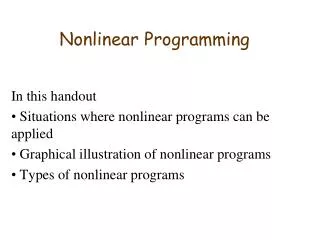
EOQ and Multiple Items • Most inventory systems stock many items • May treat each item individually and then add them up • Restrictions may be imposed (limited warehouse capacity, upper limit on the maximum dollar investment, number of orders per year, and so on) • Will be covered after covering NLP
Overview of NLP • Many realistic problems have nonlinear functions • When LP problems contain nonlinear functions, they are referred NLP • Have a separate name, because they are solved differently • In LP, solutions are found at the intersections • In NLP, there may no corner point • Solution space can be undulating line or surface • Like a mountain range with many peaks and valleys • Optimal point at the top of any peak or at the bottom of any valley • In NLP, we have local and global points
Local and Global Optimal Point • Solution techniques generally search for high points or low points • Difficulty of NLP is to determine whether the identified is a local or global optimal point • Global optimal point can be found by the very complex mathematical techniques Global optimal point Local optimal points
Constrained and UnconstrainedOptimization • Constrained optimization • Profit function: Z= vp-cf-vcv, v=1500-24.6p, cf=$10,000 and cv=$8 • vp creates a curvilinear relationship • Results in quadratic function: Z= 1696.8p-24.6p2-22,000 • δZ/δp=0, 1696.8-49.2p=0, p=34.49 • Called classical unconstrained optimization profit price
Constrained Optimization Max Z= 1696.8p-24.6p2-22,000 s.t. p<=20 • Referred NLP • Solution is on the boundary formed by constraint • Change RHS from 20 to 40 • Solution is no longer on the boundary • Makes process of finding optimal solution difficult, particularly, with more variables and constraints Feasible space P=20 price Feasible space price P=40
Single Facility Location Problem • Locate a centralized facility that serves several customers • Minimize the total miles traveled between the facility and all customers • Locations of the cities and the number of trips are: (20,20,75), (10,35,105), (25,9,135), (32,15, 60), (18,8,90) • d=[(xi-x)2+(yi-y)2]1/2 • Min Σditi city1 city3 city5 city4 city2
NLP with Multiple Constraints • Consider a problem with two constraints • A company produces two products and the production is subject to resource constraints • Demand of each product is dependent on the price (x1=1500-24.6p1 and x2=2700-63.8p2) • Cost of producing x1 and x2 are 12 and 9 • Production resources are (2x1+2.7 x2<=6000, 3.6x1+2.9x2<=8500, 7.2x1+8.5 x2<=15,000) • Model: Max z=(p1-12)x1+(p2-9)x2 s.t. 2x1+2.7 x2<=6000 3.6x1+2.9x2<=8500 7.2x1+8.5 x2<=15,000 • Where x1=1500-24.6p1 and x2=2700-63.8p2 • Decision variables are?
Solution Techniques • Very complex • Two method • Least or Substitution method • Transferring a constraint optimization to an unconstraint optimization • Lagrange multiplier
Substitution Method • Restricted to models containing only equality constraints • Involves solving the constraint for one variable for another • New expression will be substituted into the objective function to eliminate it completely
Example • Max Z= vp-cf-vcv s.t. v=15,00 -24.6 p • cf=$10,000 and cv=$8 • vp creates a curvilinear relationship • Constraint has been solved v for p • Substitute it in objective function Z= 1500p-24.6p2-cf-1500cv+24.6 pcv Z= 1696.8p-24.6p2-22,000 • Differentiating and setting it equal to zero • 0=1696.8-49.2p • p=34.49
Example • Consider the Furniture Company • Assume contribution of each declines as the quantity increases • Relationship for x1: $4-0.1x1 • Relation for x2: $5-0.2 x2 • Profit earned form each:($4-0.1x1)x1 and ($5-0.2 x2)x2 • Total profit: z=4x1+5x2-0.1x12-0.2x22 • Consider just one constraint: x1+2x2=40 or x1=40-2x2 • z=4(40-2x2)+5x2-0.1 (40-2x2)-0.2x22 • z=13x2-0.6x22 • x1=18.4, z=$70.42
Limitation of Substitution • Highest order of decision variable was a power of two • Dealt only with two decision variables and single constraint
Lagrange Multiplier • Used for constraint optimization consisting of nonlinear objective function and constraints • Transform objective function into a Lagrangian function • Constraints as multiples of Lagrange multipliers are subtracted from the objective function • Consider an example Max z=4x1+5x2-0.1x12-0.2x22 s.t. x1+2x2=40 • Forming Lagrangian function L=4x1+5x2-0.1x12-0.2x22 - (x1+2x2-40)
Lagrange Multiplier-Cont. • Partial derivatives of L with respect to each of variables • δL/δx1=0, δL/δx2=0, δL/δ=0 • 4-0.2x1=0, 5-0.4-2=0, x1-2x2+40=0 • X1=18.3, x2=10.8, =0.33, z=70.42
Sensitivity Analysis • Lagrangian multiplier, , is analogous to dual variables in LP • Shows changes in objective function value by changing the RHS • Positive value of shows the increase in objective function • Example Max z=4x1+5x2-0.1x12-0.2x22 s.t. x1+2x2=41 • x1=18.8, x2=11.2, =0.27, z=70.75
Mathematical Notations • Di=Annual demand for item i in units • Ci=Unit purchase cost of item i in dollar • Ai= ordering cost of item i in dollar • fi=Required storage space for item i in square foot • F=Maximum total storage space available • TC=Total average annual costs in dollar • Hi= Annual holding cost per unit i per year in dollar
Example-Limited Working Capital Total=17120 Available budget=15,000 Inventory carrying charge=0.2
Solution • Solved by the method of Lagrange‑multiplier • Before applying the method, we should solve the total cost function by ignoring the constraint • Otherwise, we form the Lagrangian expression
Lagrangian Expression • Total budget=17120> available budget=15000 • Form the Lagrangian Expression • Derivative with respect to Qi and lambda
Final Result • From the first equation • From the second equation
HW Assignment #1 • Assume that the annual inventory carrying charge is 10% • and that 15000 sq.ft of floor space are available. • What is the optimal inventory policy for these items. • Determine the cost of having only 15,000 sq.ft of floor space?
HW#2 Classify these items into A, B, and C.
HW#3 • The Furniture Company has developed the following NLP model to determine the optimal number of chairs and tables to produce daily. Max z=7x1-0.3x12 +8x2-0.4x22 S.t. 4x1+5x2=100 hr • Determine the optimal solution to this NLP using the substitution method. • Determine the optimal solution to this NLP using the Lagrange multipliers.
HW#4 • Consider the following NLP model to determine solution. Max z=30x1-2x12 +25x2-0.5x22 S.t. 3x1+6x2=300 • Determine the optimal solution to this NLP using the substitution method. • Determine the optimal solution to this NLP using the Lagrange multipliers.
HW#5 • Section 11.2c, Problems 1 and 4