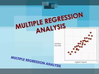
1. Nonlinear and multiple regression analysis Just a straightforward extension of linear regression analysis

2. Let’s look at our demand data that we used to estimate a linear relationship We can easily transform these data to their natural logarithms by using the formula Ln( ) in other ranges of cells but inserting the original cell addresses of the absolute value data in the natural logarithm formula and then copying down columns Now we are transforming the linear model, Y = a + bX to the loglinear model, Ln(Y) = Ln(a) + bLn(X), or this latter model can be written in nonlinear form as Y=AXb And we can use the Excel regression tool to estimate such a model

3. Our new demand relationship will be shaped similar to the demand curve in the graph below, depending now on our estimates of A = antilog(a), and b from the model y=AXb, where Y = quantity purchased and X = price, with parameters A and b Price Quantity

4. Now let’s show both our original quantity-price data for the 12 observations and the logarithmic data Next, we input the logarithmic data into the regression tool, much the same way as we did the original data in absolute value, i.e., we input the Y-input data or the quantities, and then the X-input data or the prices with quantities being the dependent variable and price being the independent variable Then view the regression analysis results

5. Notice the results --- the estimate of the price coefficient is negative at – 2.61 rounded, and our estimate of the intercept term is going to be very large by taking EXP(13.68) --- the R2 value is slightly lower than in the linear case, and the F-Statistic significance is a bit higher But, the t-ratios in absolute value give us confidence that this model is not by any means an erroneous model of the demand conditions of our data ---- the goodness of fit is slightly less than the linear case

6. A finance problem • Now for you finance buffs, let’s go to a finance problem where we relate the returns of a company to the returns of the 90-day Treasuries (U.S.) and the market reflected by the Standard & Poors (S&P) returns • Our model is then ri = a + bTi + c(S&P)i • Where ri = a companies returns, Ti = treasuries returns, and (S&P)i = stock market return • The parameters of the model are a, b and c, with a = intercept term, and b and c are, respectively, the treasuries return slope and the S&P return slope

7. Below is our data set of returns for the company (called slow stock retuern), the treasuries return and the return of the market { the S&P} We can use the regression tool again to get an estimate of this model, but notice we have a multiple regression problem We are going to regress the dependent variable, slow stock retuern, and 2 independent variables, treasuries return and S&P index. We input the dependent, or Y-input cells as the cells containing Slow Stock Retuern, and then we input the X-input cells as both the Treasuries and S&P returns --- we can just drag both columns into the X-input window

8. We can check labels, since we have the names of both independent variables and the single dependent variable, and the independent variables will then be identified in the analysis of variance results ---- then click OK, to get the following regression model There does not appear to be a strong relationship between Slow Stock retuern rates of return and the treasuries and market returns as represented by this model Notice that the R2 value is considerably less than we obtained in the previous demand model regressions --- But notice also we have rather low t-ratios for each the two explanatory (independent variables --- there is a higher chance that these coefficients are zero--- indicating they are not statistically different from zero

9. We can also develop a model of the Capital Asset Pricing Model with these data Recall, for those of you who have had some finance training like completing Economics 5600, the capital asset pricing model (CAPM) is derived as ri = rf + (rm – rf), where ri = the individual stock company return, rm = the return of the market, such as the S&P return, and rf = the risk free return, or near risk free return such as the interest rate on 90-day Treasury bills. The parameter  is the slope of the CAPM system and is defined, from our experience in finance as  = [covariance of security i’s return with the return of the market (like the S&P index)] / [variance of market (S&P) returns] Using the CAPM we can then relate returns to the individual company to the market and find the Beta () for that particular companies returns which tells us whether these individual company returns move with the market or have no relationship to market returns. Recall, if  < 1, then the company returns are considered less risky that the returns of the market. If  = 1, the company returns move in lock step with returns in the market, and if  > 1, then company returns bear greater risk than returns from the general stock market. So we would want to find out which case exists by estimating the parameter  using the CAPM relationship given above.

10. Hence, we can find the values (rm – rf), which are the excess returns of the market over the risk free rate of return, which then becomes our independent variable We then regress the individual company returns on this excess returns variable to get an estimate of  Again we can use the regression tool in Excel to derive our estimate The data of this conversion are given below

11. The regression of Slow stock Retuern company stock returns on the excess returns is given below If we had a statistically significant  from this estimate at the value shown below of 0.2397, this would indicate that company returns are less risky than returns from the general stock market ---- but we do not have strong statistical properties of the relationship Notice that the t-ratios have improved just slightly --- the estimated  is 0.2397 but this estimate does not have a t-ration at 1.96 or greater --- therefore, the beta value is not significantly different from zero statistically Hence again, we do not have a good relationship between company returns and the return of the market. They are not moving together in returns or cash flow from which the returns are derived.

12. We can also develop an estimate of  by using the embedded statistical functions of Excel Notice that  = [covariance of company returns with returns of the market] all divided by [the variance of returns of the market] So we could use the commands, COVAR (cell range of company returns, cell range of S&P returns) / VAR(S&P returns) to get the value of  right in Excel COVAR is the command for covariance, and VAR is the command to compute variance We could also derive  using the Excel command, SLOPE, by just entering this command as SLOPE (range of cells of company returns, range of cells of S&P returns), since  is the slope of the CAPM model indicating how company returns will change as excess returns change Of course, we would not get all the statistical properties that we would want in this case, but we can get a quick estimate You may want to try other regression estimation models to give yourself experience in using Excel to estimate regression equations and use other Excel functions and commands