Bayesian Inference of Binomial Problems for Estimating Success Probabilities
This document outlines the process of Bayesian inference for estimating the unknown proportion of success (or probability) from binomial data acquired through Bernoulli trials, consisting of outcomes of 0s and 1s. It begins with defining the parameter q as the success proportion and utilizing the binomial distribution for analysis. Various examples, including real-world applications like estimating female birth probabilities, are explored with non-informative and informative priors. The document provides practice exercises using MATLAB for plotting distributions and calculating posterior predictions.

Bayesian Inference of Binomial Problems for Estimating Success Probabilities
E N D
Presentation Transcript
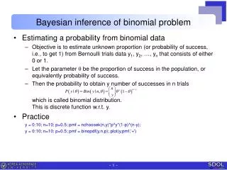
Bayesian inference of binomial problem • Estimating a probability from binomial data • Objective is to estimate unknown proportion (or probability of success, i.e., to get 1) from Bernoulli trials data y1, y2, …, yn that consists of either 0 or 1. • Let the parameter q be the proportion of success in the population, or equivalently probability of success. • Then the probability to obtain y number of successes in n trials which is called binomial distribution.This is discrete function w.r.t. y. • Practice y = 0:10; n=10; p=0.5; pmf = nchoosek(n,y)*p^y*(1-p)^(n-y); y = 0:10; n=10; p=0.5; pmf = binopdf(y,n,p); plot(y,pmf,'+')
Bayesian inference of binomial problem • Inference problem statement • Let the parameter q be the proportion of females in the population. • Current accepted value in Europe is 0.485, less than 0.5. • Estimate q conditional on the observed data: y females out of n births. • Simplest way is just to let q = y/n. • Bayesian inference • Assume non-informative prior: q ~ uniform on [0, 1]. • Likelihood: • Posterior density:
Bayesian inference of binomial problem • Illustrative results • Several different experiments but with same proportion of successeswhere sample sizes vary. • Interpret the meaning of the figures. • Practice: plot the four cases using matlab function.
Bayesian inference of binomial problem • Beta pdf • In fact, the posterior density is beta distribution with parameters a = y+1, b = n-y+1. • Practice : plot the four cases using beta pdf function. • Laplace in 18th Century • 241,945 girls, 251,527 boys in Paris during 1745 ~ 1770. • P[q ≥ 0.5 | y] ≈ 1.1510-42 So he was ‘certain’ that q < 0.5. • Practice: calculate this value, and validate. • Posterior prediction • What is the probability to get girl if a new baby born ? • Practice: calculate this value. What if the numbers were 2 out of 5 ?
Bayesian inference of binomial problem • Summarizing posterior inference • Locations summary: • Mean: expectation, needs integration. • Mode: most-likely value. Maximum of pdf. Needs optimization or d(pdf)/dx. • Median: 50% percentile value. • Among these, mode is preferred due to the computational convenience. • Variations summary: • Standard deviation or variance • Interquartile range or 100(1-a)% interval • Practice with beta pdf.Mean, mode are given as equation analytically.Others are obtained using matlab functions. • In general, these values are computed using computer simulations from the posterior distribution.
Bayesian inference of binomial problem • Informative prior • So far considered only uniform prior. • Recall the likelihood is binomial pdf: • Let us introduce prior of beta pdf: where a, b are called hyperparameters. • Then posterior density: • Remarks • Property that posterior distribution follows same form as the prior is called conjugacy. Beta prior is conjugate family of binomial likelihood. • As a result, the mean & variance of posterior pdf: • As y & n-y become large under fixed a & b,In the limit, parameters of the prior have no influence on posterior.Besides, it converges to normal pdf due to central limit theorem.
Homework • 2.5 example: estimating probability of female birth • P[ q < 0.485 ] • Histogram of posterior pdfq|y • Median and 95% confidence intervals. Ans .446, [.415, .477]