Download
1 / 50
510 likes | 699 Vues
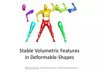
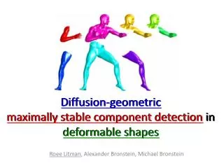
Diffusion-geometric maximally stable component detection in deformable shapes. Diffusion- geometric maximally stable component detection in deformable shapes. Roee Litman , Alexander Bronstein , Michael Bronstein. In a nutshell…. The Feature Approach for Images.

E N D
Diffusion-geometricmaximally stable component detection in deformable shapes Diffusion-geometricmaximally stable component detection in deformable shapes Roee Litman, Alexander Bronstein, Michael Bronstein
In a nutshell… The Feature Approach for Images Deformable Shape Analysis MSER Maximally Stable ExtremalRegion Diffusion Geometry Shape MSER
Feature Approach in Images Feature based methods are the infrastructure laid in the base of many computer vision algorithms: • Content-based image retrieval • Video tracking • Panorama alignment • 3D reconstruction form stereo
Problem formulation • Find a semi-local feature detector • High repeatability • Invariance to isometric deformation • Robustness to noise, sampling, etc. • Add discriminative descriptor
The “what” Results
More Results (Taken from the TOSCA dataset) Horse regions + Human regions
Region Matching Query 1st, 2nd, 4th, 10th, and 15th matches
3D Human Scans Taken from the SCAPE dataset
Scanned Region Matching Query 1st, 2nd, 4th, 10th, and 15th matches
Volume vs. Surface Original Volume & surface isometry Boundary isometry
Volumetric Shapes • Usually shapes are modeled as 2D boundary of a 3D shape. • Volumetric shape model better captures "natural" behavior of non-rigid deformations.(Raviv et-al) • Diffusion geometry terms can easily be applied to volumes • 2D Meshes can be voxelized
Volumetric Regions Taken from the SCAPE dataset
(The “how”) Methodology
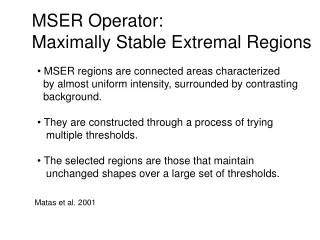
MSER • Popular image blob detector • Near-linear complexity: • High repeatability [Mikolajczyk et al. 05] • Robust to affine transformation and illumination changes
MSER – In a nutshell • Threshold image at consecutive gray-levels • Search regions whose area stay nearly the same through a wide range of thresholds • Efficient detection of maximally stable regions requires construction of a component tree
Algorithm overview • Represent as weighted graph • Component tree • Stable component detection
Algorithm overview • Represent as weighted graph
Image as weighted graph • An undirected graph can be created from an image, where: • Vertices are pixels • Edges by adjacency rule, e.g. 4-neiborhood
Weighting the graph In images • Gray-scale as vertex-weight • Color as edge-weight [Forssen] In Shapes • Curvature (not deformation invariant) • Diffusion Geometry
Weighting Option • For every point on the shape: • Calculate the prob. of a random walk to return to the same point. • Similar to Gaussian curvature • Intrinsic, i.e. – deformation invariant
Weight example Color-mapped Level-set animation
Diffusion Geometry • Analysis of diffusion (random walk) processes • Governed by the heat equation • Solution is heat distributionat point at time
Heat-Kernel • Given • Initial condition • Boundary condition, if these’s a boundary • Solve using: • i.e. - find the “heat-kernel”
Probabilistic Interpretation The probability density for a transition by random walk of length , from to
Spectral Interpretation • How to calculate ? • Heat kernel can be calculated directly from eigen-decomposition of the Laplacain • By spectral decomposition theorem:
Computational aspects • Shapes are discretized as triangular meshes • Can be expressed as undirected graph • Heat kernel & eigenfunctions are vectors • Discrete Laplace-Beltrami operator • Several weight schemes for • is usually discrete area elements
Computational aspects • In matrix notation • Solve eigendecomposition problem
Auto-diffusivity • Special case - • The chance of returning to after time • Related to Gaussian curvature by • Now we can attach scalar value to shapes!
Weight example Color-mapped Level-set animation
Algorithm overview • Represent as weighted graph • Component tree • Stable component detection
The Component Tree • Tree construction is a pre-process of stable region detection • Contains level-set hierarchy,i.e. nesting relations. • Constructed based on a weighted graph (vertex- or edge-weight) • Tree’s nodes are level-sets(of the graph’s cross-sections)
“Graphic” Example • A graph • Edge-weighted • 7 Cross-Section • 5 Cross-section • Two 5 level-sets(with altitude 4) • Every level-set has • Size (area) • Altitude (maximal weight) 4 7 8 9 8 1 4 1
Tree Construction 4 4 7 7 8 8 9 9 8 8 1 1 4 4 1 1
Algorithm overview • Represent as weighted graph • Component tree • Stable component detection
Detection Process • For every leaf component in the tree: • “Climb” the tree to its root, creating the sequence: • Calculate component stability • Local maxima of the sequenceare “Maximally stable components”
The Detils Performance
Benchmarking The Method • Method was tested on SHREC 2010 data-set: • 3 basic shapes (human, dog & horse) • 9 transformations, applied in 5 different strengths • 138 shapes in total Scale Original Deformation Holes Noise
Quantitative Results • Vertex-wise correspondences were given • Regions were projected onto another shape, and overlap ratio was measured • Overlap ratio between a region and its projected counterpart is • Repeatability is the percent of regions with overlap above a threshold
Repeatability 65% at 0.75
Conclusion • Stable region detector for deformable shapes • Generic detection framework: • Vertex- and edge-weighted graph representation • Works on surface and/or volume data • Partial matching & retrieval potential • Tested quantitatively (on SHREC10)
Thank You Any Questions?