MAXIM Periscope Module
MAXIM Periscope Module. PRICE H Cost Modeling Bill Lawson 25 April 2003. PRICE H Cost Model. PRICE H: Commercial Parametric Hardware Cost Modeling Tool Tool Heritage: DOD Global Parameters: Labor Costs: GSFC bid rates (used for in-house builds of spacecraft/instrument)

MAXIM Periscope Module
E N D
Presentation Transcript
MAXIM Periscope Module PRICE H Cost Modeling Bill Lawson 25 April 2003
PRICE H Cost Model • PRICE H: Commercial Parametric Hardware Cost Modeling Tool • Tool Heritage: DOD • Global Parameters: • Labor Costs: GSFC bid rates (used for in-house builds of spacecraft/instrument) • Inflation: NASA Inflation Index (MAXIM costs presented in Constant 2003 dollars) • Engineering Environment • NASA environment defined by PRICE Systems, Inc. calibration study • Baseline environment emphasizes System Engineering, Project Management, and automated design capabilities • Key Component Parameters: • Complexity Factors (Table driven from industry experience) • Modification Level/Remaining Design Factor (Heritage) • Quantity and Design Repeat (Learning Curve) • Composition (Structure, Electronic, Purchased, Cost Pass-through) • Mass • Operating Platform (Unmanned-Space)
ISAL PRICE H Cost Modeling • Study begins with a blank model • Instrument payloads vary making a template approach difficult • Similar components (e.g., electronics) from prior studies were incorporated and modified • ISAL study output products: • Powerpoint presentation • PRICE H model exported to Summary Excel Spreadsheet • PRICE H model exported to Detailed Excel Spreadsheet • PRICE model file (requires PRICE H software) • Upon request: Text reports containing input/outputs for each cost element
PRICE Cost Summary1st “Periscope-Pair” Cost Element (Summary Report Available for each cost element) Engineering Year Dollars ($03) Project Management Production Manufacturing Development Total Cost Estimate $23.9M Schedule Mass
Total Cost (incremental cost for T2 is $2.24M) PRICE Cost Estimate Summary Incremental Cost of 2nd Unit (T2) T1 T1 + T2
Learning Curve Basics • PRICE H Users Manual: • Basis for improvement is the “human learning process” • Learning curves in PRICE H apply to production run (not development) • The more one produces, the more efficient one becomes • Production learning improvement is virtually non-existent for automated manufacturing methods • PRICE H provides a parameter to adjust the degree of automation (MPI) • Typically, automation lowers Theoretical First Piece (T1) cost and flattens the Unit Learning Curve • NASA Cost Estimating Handbook (April 2002) • The learning curve concept is used primarily for uninterrupted manufacturing and assembly tasks • The major premise of learning curves is that each time the product quantity doubles the resources (labor hours) required to produce the product will reduce by a determined percentage.
Multiple Unit Studies (PRICE H Learning Curve) • PRICE H: • Calculates Theoretical First Piece (T1) production unit (most costly to produce) • Incorporates industry standard Boeing Unit Learning Curve (ULC) • Applies a correction factor to improve accuracy (for lower quantity studies) • Includes Stanford-b formula to transfer prototype learning to manufacturing • Calculates Production Average Unit Cost (UPC) A A (QTY + QCF + Stan_b) - (QCF + Stan_b) Production Cost = T1 - ULCF A Where: (A – 1) (A – 2) ULCF is PRICE H correction factor ULCF = 24 ln(UNITLC) Part of Boeing Equation A = 1 + ln(2) Quantity dependent correction factor QCF = 0.5151 – 0.001116 ln(QTY) Stan_b = (input %)(Protos) Percent of Prototypes to include
MAXIM_PRICEcost.xlsDetailed Cost Estimate (1st “Periscope-Pair”) …


