Chapter 11 : Linear Regression

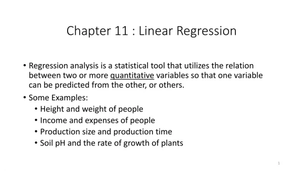
1. Chapter 11 : Linear Regression • Regression analysis is a statistical tool that utilizes the relation between two or more quantitative variables so that one variable can be predicted from the other, or others. • Some Examples: • Height and weight of people • Income and expenses of people • Production size and production time • Soil pH and the rate of growth of plants

2. Correlation • An easy way to determine if two quantitative variables are linearly related is by looking at their scatterplot. • Another way is to calculate the correlation coefficient, denoted usually by r. • The Linear Correlation measures the strength of the linear relationship between explanatory variable (x) and the response variable (y). An estimate of this correlation parameter is provided by the Pearson sample correlation coefficient, r. Note: -1 ≤ r ≤ 1.

3. Example Scatterplots with Correlations If X and Y are independent, then their correlation is 0.

4. Correlation If the correlation between X and Y is 0, it doesn’t mean they are independent. It only means that they are not linearly related. • Some Guidelines in Interpreting r. One complain about the correlation is that it can be subjective when interpreting its value. Some people are very happy with r≈0.6, while others are not. Note: Correlation does not necessarily imply Causation!

5. Simple Linear Regression Y=β0+β1x Random Error • Model: Yi=(β0+β1xi) + εi where, • Yi is the ith value of the response variable. • xi is the ith value of the explanatory variable. • εi’s are uncorrelated with a mean of 0 and constant variance σ2. • How do we determine the underlying linear relationship? • Well, since the points are following this linear trend, why don’t we look for a line that “best” fit the points. • But what do we mean by “best” fit? We need a criterion to help us determine which between 2 competing candidate lines is better. * Observed point y * * * * ε1 * * L4 * Expected point L3 x1 x L2 L1

6. Method of Least Squares Y=β0+β1x • Model: Yi=(β0+β1xi) + εi where, • Yi is the ith value of the response variable. • xi is the ith value of the explanatory variable. • εi’s are uncorrelated with a mean of 0 and constant variance σ2. • Residual = (Observed y-value) – (Predicted y-value) e1= y1 – y * Observed * P1(x1,y1) Predicted Example: 2+.8x * * y1 * e1 * * e2 * x1 x Method of Least Squares: Choose the line that minimizes the SSE as the “best” line. This line is unknown as the Least-Squares Regression Line. Question:But there are infinite possible candidate lines, how can we find the one that minimizes the SSE? Answer: Since SSE is a continuous function of 2 variables, we can use methods from calculus to minimize the SSE.

7. Model Assumptions • Model: Yi=(β0+β1xi) + εi where, • εi’s are uncorrelated with a mean of 0 and constant variance σ2ε. • εi’s are normally distributed. (This is needed in the test for the slope.) Y=β0+β1x Since the underlying (green) line is unknown to us, we can’t calculate the values of the error terms (εi). The best that we can do is study the residuals (ei). Observed point y * e1 ε1 Expected point Predicted point x1 x