Conceptual Design Review for PRIMA

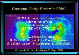
1. Conceptual Design Review for PRIMA Frosty Leo CW Leo PRIMA Astrometric Observations Polarization effects Technical Report AS-TRE-AOS-15753-0011 Koji Murakawa (ASTRON) B. Tubbs, R. Mather, R. Le Poole, J. Meisner, E. Bakker (Leiden), F. Delplancke, K. Scale (ESO) @Lorentz Center, Leiden on 29 Sep., 2004

2. - OUTLINE - 1. Introduction Why instrumental polarization analysis? 2. Effects of phase error on astrometry Operation principle of the FSU 3. Polarization properties of PRIMA optics Basic concepts of polarization model

3. Introduction • Why instrumental polarization analysis? • changes phase and amplitude VLT telescope, StS, base line, etc (telescope pointing, separation, station…) • the fringe sensor unit detects a wrong phase delay. • provide an error in astrometry what kind of error? (<p/100?)

4. What we have to do? • Establish a strategy of analysis • Study the operation principle of FSU • Make a polarization model of VLTI optics Analysis • Fringe detection by FSU • polarization model analysis of VLTI optics • telescope, StS, base line optics • time evolution (as a function of hour angle) • difference between the ref. and the obj.

5. The Operation Principleof the Fringe Sensor Unit Alenia Co., VLT-TRE-ALS-15740-0004

6. The original ABCD Algorithm Complex Amplitude EA = -b(P1-P2) EB = b(S1+S2) EC = b(P1+P2) ED = -b(S1-S2) Identical polarization S1 = expi(kLopl,1) S2 = expi(kLopl,2) P1 = expi(kLopl,1) P2 = expi(kLopl,2 +p/2) k: wave number (k=2p/l) Lopl,i: optical path length at the station i

7. The original ABCD Algorithm ABCD signals IA = 2|b|2{1+sin(kLopd)} IB = 2|b|2{1+cos(kLopd)} IC = 2|b|2{1-sin(kLopd)} ID = 2|b|2{1-cos(kLopd)} Visibility V = 1/2(IA+IB+IC+ID)=4|b|2 Phase delay f = kLopd = arctan(IA-IC/IB-ID) Lopd: optical path difference Lopd = Lopl,1 - Lopl,2 The phase delay can be measured with a simple way.

8. The original ABCD Algorithm Complex Amplitude EA = -b(P1-P2) EB = b(S1+S2) EC = b(P1+P2) ED = -b(S1-S2) Different polarization S1 = S1expi(kLopl,1) S2 = S1expi(kLopl,2) P1 = P1expi(kLopl,1) P2 = P1expi(kLopl,2+p/2) k: wave number (k=2p/l) Lopl,i: optical path length at the station i

9. The original ABCD Algorithm ABCD signals IA = 2|bP1|2{1+sin(kLopd)} IB = 2|bS1|2{1+cos(kLopd)} IC = 2|bP1|2{1-sin(kLopd)} ID = 2|bS1|2{1-cos(kLopd)} Visibility V = 1/2(IA+IB+IC+ID) = 2|b|2(|P1|2+|S1|2) Phase delay f = kLopd = arctan(IA-IC/IA+IC * IB+ID/IB-ID) Lopd: optical path difference Lopd = Lopl,1 - Lopl,2 The phase delay can be measured not affected by different polarization status between S and P.

10. A Modified ABCD Algorithm Complex Amplitude EA = -b(P1-P2) EB = b(S1+S2) EC = b(P1+P2) ED = -b(S1-S2) Different polarization S1 = S1expi(kLopl,1) S2 = S2expi(kLopl,2) P1 = P1expi(kLopl,1+fS) P2 = P2expi(kLopl,2+fP+p/2) • Different polarization between beam 1 and 2 • phase fS = fS,2-fS,1, and fP = fP,2-fP,1 • amplitude S2≠S1, P2≠P1

11. A Problem on the ABCD Algorithm ABCD signals IA = |b|2{P12+P22+2P1P2sin(kLopd+fP)} IB = |b|2{S12+S22+2S1S2cos(kLopd+fS)} IC = |b|2{P12+P22-2P1P2sin(kLopd+fP)} ID = |b|2{S12+S22-2S1S2cos(kLopd+fS)} The ABCD algorithm tells a wrong phase delay.

12. A Modified ABCD Algorithm Get another sampling with a p/2(=l/4) step IA0 = |b|2{P12+P22+2P1P2sin(kLopd+fP)} IA1 = |b|2{P12+P22+2P1P2cos(kLopd+fP)} IC0 = |b|2{P12+P22-2P1P2sin(kLopd+fP)} IC1 = |b|2{P12+P22-2P1P2cos(kLopd+fP)} • only P-polarization is described above. • assume fixed P1 and P2

13. A Modified ABCD Algorithm& Polarization Effects Phase delay FP = kLopd + fP = arctan(IA0-IC0/IA1+IC1) FS = kLopd + fS = arctan(IB0-ID0/IB1+ID1) The FSU may correct (detect) 1/2(FP+FS) = kLopd+1/2(fP+fS) • Instrumental polarization between two beams • cannot be principally corrected. • a phase delay of |fS-fP| still remains.

14. Impact on Astrometry- Polarization Effects on Object - Visibility of the object V = <|ES,1+ES,2+EP,1+EP,2|2> = <|ES,1|2>+<|ES,2|2>+<|EP,1|2>+<|EP,2|2> +<ES,1ES,2*>+<ES,1*ES,2> +<ES,1EP,1*>+<ES,1*EP,1> +<ES,1EP,2*>+<ES,1*EP,2> +<ES,2EP,1*>+<ES,2*EP,1> +<ES,2EP,2*>+<ES,2*EP,2> +<EP,1EP,2*>+<EP,1*EP,2> ES,1 = S1expi(kLopl,1’) ES,2 = S2expi(kLopl,2’+fS’) EP,1 = P1expi(kLopl,1’+fSP’) EP,2 = P2expi(kLopl,2’+fSP’+fP’)

15. Impact on Astrometry- Polarization Effects on Object - Cross correlation <ES,1ES,2*>+<ES,1*ES,2> = 2S1S2<cos(klopd’-fS’)> <ES,1EP,1*>+<ES,1*EP,1> = 2S1P1<cos(fSP’)> <ES,1EP,2*>+<ES,1*EP,2> = 2S1P2<cos(klopd’-fSP’-fP’)> <ES,2EP,1*>+<ES,2*EP,1> = 2S2P1<cos(klopd’+fSP’-fS’)> <ES,2EP,2*>+<ES,2*EP,2> = 2S2P2<cos(fSP’+fP’-fS’)> <EP,1EP,2*>+<EP,1*EP,2> = 2P1P2<cos(klopd’-fP’)>

16. Impact on Astrometry- Polarization Effects on Object - Visibility of the unpolarized object V = <|ES,1+ES,2+EP,1+EP,2|2> = <|ES,1|2>+<|ES,2|2>+<|EP,1|2>+<|EP,2|2> +2<S1S2cos(klopd’-fS’)>+2<P1P2cos(klopd’-fP’)> Because of <cos(fSP’)>=0….unpolarized light Astrometry of the unpolarized object k(Lopd-Lopd’)+{(fS-fP)-(fS’-fP’)} = kLBLsinq+{(fS-fP)-(fS’-fP’)} … q: astrometry

17. Impact on Astrometry- Summary - • Operation principle of FSU • Phase delay measurement not affected by polarization status of the reference. • A modified ABCD algorithm to calibrate instrumental polarization 2. Impact on astrometry • {(fS-fP)-(fS’-fP’)} gives error in astrometry • Similar beam combiner to the FSU is encouraged to science instrument

18. Polarization Model Optics can work as a phase retarder or a polarizer So = JSi … S: Stokes parm, J: Jones matrix Sf = JNJN-1…J1 S* Grouping Jtel(Az(h), El(h), r, q, l, St): telescope optics JStS(r, q, l): star separator optics JBL(l, St): base line optics Model Sf = JBLJStSJtelS*

19. Future Activities 1. Telescope optics (Jtel) time evolution: |fS-fP|(h, Dec, r, q) 2. Star separator optics (JStS) |fS-fP|(r) 3. Base line optics (JBL) |fS-fP|(St) 4. Color dependence fopd(l), Ix(l)@FSU, group delay