Cooperative TSP
This presentation explores Cooperative Traveling Salesman Problems (cTSP), where customers assist the salesperson in minimizing delivery routes. We delve into various cooperation modes—purchase, sales, and full cooperation—alongside minimization goals such as Min-Sum, Min-Max, and Min-Makespan. Examples, including secret distribution and waking robots, demonstrate practical applications. We also present our results, which include constant-factor approximations and polynomial-time algorithms, while addressing the algorithmic complexities and hardness of cTSP variations.

Cooperative TSP
E N D
Presentation Transcript
Cooperative TSP Amitai Armon, Adi Avidor and Oded Schwartz Tel-Aviv University, Israel
Presentation Overview • Introducing Cooperative TSP problems • Cooperation modes • Minimization goals • Examples • Our results and related results • Outline of one of our PTAS algorithms
Classical TSP A salesperson has to deliver goods to a set of customers, while minimizing the total travel. 2 4 3 5 1 2 3 5 5 3 2 2 1 1 1 3 3 4 2
Cooperative TSP (cTSP) The customers cooperate with the salesperson, and can move to help in the deliveries. 2 4 3 5 1 2 3 5 5 3 2 2 1 1 1 3 3 4 2
General Motivation In many realistic cases, all the participants are on the same side: The “customers” are actually other agents of the same organization. 2 4 3 5 1 2 3 5 5 3 2 2 1 1 1 3 3 4 2
Cooperation Modes The agents (customers) may help in one of the following ways: • Purchase-cooperation: The agents can be instructed to move in order to receive the goods. • Sales-cooperation: The agents can be instructed to distribute the goods after receiving them. • Full-cooperation: Both 1 and 2. (We assume all the agents cooperate in the same mode)
Minimization Goals The following goals are considered: • Min-Sum: Minimizing the totaldistance traveled by all the participants. • Min-Max: Minimizing the maximaldistance traveled by any participant. • Min-Makespan: Minimizing the time required for completing the deliveries.
The Way Back: Two Versions • In the “Roundtrip” version, each participant must return to his/her starting-point at the end of the process. • In the “Path” version, we are only interested in what happens until all the deliveries are made.
Example: Distributing a secret to spies • A secret should be distributed in person to all the spies as soon as possible. • Each spy is instructed where and when to receive it. • Spies who receive the secret can be instructed to help in further distributing it. PathMin-Makespan Full-Cooperation cTSP
Example: Waking-up robots • Sleeping robots need to be awaken. • Each awake robot can help in waking-up the others (initially one robot is awake). • Each robot has limited battery, and thus should travel as little as possible. Path Min-Max Sales-Cooperation cTSP
Example: Distributing Cash • A secured car distributes cash from the bank’s headquarters to its branches. • Each branch can be instructed to send a car to meet it and take its own part. • The bank wishes to minimize the total travel (or the total travel of cash-loaded cars). Roundtrip/Path Min-Sum Purchase-Cooperation cTSP
The Metric Space We consider both: • A general metric space: a weighted undirected graph satisfying the triangle inequality. • A fixed-dimension Euclidean space (we refer to this problem as “Euclidean cTSP”).
The Scope of this Work • We consider all the combinations of the problems mentioned: Cooperation-mode x Minimization-goal x Roundtrip/Path x Euclidean/graph (Except for versions which have already been considered, as described later). • We provide both algorithmic and hardness results.
Presentation Overview • Introducing Cooperative TSP problems • Cooperation modes • Minimization goals • Examples • Our results and related results • Outline of one of our PTAS algorithms
Previous Results Classical metric TSP: • In graphs: 3/2 approximation[Christofides 1976, Hoogeveen 1991] No approximation < 203/202 [Engebretsen and Karpinski 2001] • In fixed-dimension Euclidean space: PTAS [Arora 1998, Mitchell 1999] NP-hard[Papadimitriou 1977]
Previous Results The Freeze-Tag problem [ABFMS, 2002] • This is exactly Path Min-Makespan Sales cTSP (waking-up robots ASAP). • In graphs: [Konemann, Levin, Sinha 2004] No approximation < 5/3[ABFMS, 2002] • In fixed-dimension Euclidean space: PTAS [ABFMS, 2002] NP-hardness conjectured[ABFMS, 2002]
Overview of Our Results • We provide constant-factor approximations for most of the problems, PTAS for some, and polynomial-time algorithms for a few. • We also provide lower-bounds on the approximability of most of the problems, some of them match our upper bounds.
Our Results for cTSP in Graphs Purchase Cooperation Sales Cooperation Full Cooperation Approx. Inapprox. Approx. Inapprox. Approx. Inapprox. PATH Min-Sum 2+ln 3 NP-hard 2 NP-hard 2+ln 3 APX-hard Min-Max PTAS No FPTAS 3 2- 4 2- Min-Makespan Polynomial 5/3-(2) 2 2- RoundTrip Min-Sum 3/2 203/202- 3/2 203/202- 3/2 203/202- Min-Max PTAS No FPTAS 3 3/2- 2 2- Min-Makespan Polynomial 5/4- 2 2- (1) by [KLS04] (2) by [ABFMS02]
Our Results for Euclidean cTSP Purchase Cooperation Sales Cooperation Full Cooperation (1) by [ABFMS02] PATH Min-Sum PTAS 5/3+ 2+ Min-Max PTAS 3 4 Min-Makespan Polynomial PTAS1 PTAS RoundTrip Min-Sum PTAS PTAS PTAS Min-Max PTAS 3 2 Min-Makespan Polynomial PTAS PTAS
Presentation Overview • Introducing Cooperative TSP problems • Cooperation modes • Minimization goals • Examples • Our results and related results • Outline of one of our PTAS algorithms
Euclidean Path Min-Sum Purchase cTSP • Recall that in this problem: • Agents canapproach the salesperson but cannothelp in delivering the goods to others. • The total travel should be minimized. • We provide a PTAS for this problem by adapting Arora’s Euclidean-TSP technique. • The challenge is considering movements of many participants rather than one, without reaching a super- polynomial running-time.
Euclidean Path Min-Sum Purchase cTSP • We define “portals-limited-solutions”. • Their optimum can be found in polynomial time, and it can be made arbitrarily close to the global optimum. • We next outline the algorithm for the planar case.
Preliminaries • We assume w.l.o.g. that all the n participants are inside the bounding-square [0,L]2,and that OPT ≥ L, where L is the smallest power of 2 s.t. L≥ 4n2. • We divide the bounding-square into four equal squares, “super-pixels of level 1”. • We repeatedly perform this division, until we reach super-pixels of level logL (and size 1), also called “pixels”. L L
Portals • We mark each super-pixel boundary-line with m equidistant points,called “portals”. • m is the smallest power of 2 s.t. m≥4 logL / e (Q(logn / e)) • A portal of a super-pixel of leveli is also a portal of a super-pixel of leveli+1. m m
A portals-limited-solution: Requirements • A participant may cross a super-pixel boundary only at its portals. • Each participant first moves to its pixel’s center. • Deliveries are only made at pixel-centers. • If a pixel is visited by two or moreparticipants, all the agents who visit it travel to its center and stop. • The salesperson may cross her/his own tour only at a portal. There are no other crossings.
Tours in optimal portals-limited-solutions Straight segments, first connecting the starting point to the pixel-center, then connecting pixel-centers and portals.
Tours in optimal portals-limited-solutions Straight segments, first connecting the starting point to the pixel-center, then connecting pixel-centers and portals.
Optimal portals-limited-solution: Properties • Each portal is used by at most one participant. • If that participant is an agent, the portal is used once. • If that participant is the salesperson, we can assume that the portal is used at most once in each direction (by shortcutting).
Portals in portals-limited-solutions Thus, for each portal p of a given super-pixel, there are six possibilities for its usage in an optimal solution: 1. The salesperson enters the super-pixel through p 2. The salesperson leaves the super-pixel through p 3. Both 1 and 2 4. One agent enters the super-pixel through p 5. One agent leaves the super-pixel through p 6. The portal is not used (In option 5 only this agent visits that super-pixel)
Valid-lists in portals-limited-solutions • Enumerating over at most 64m combinations for the usage of portals of a super-pixel takes poly(n1/e) time. • If such a combination may be a valid part of a solution, we call it a “valid-list”. • For each valid-list there are poly(n1/e) possible pairings of entry and exit points of the salesperson in a pixel.
The PTAS: Computing optimal costs for all the valid-lists • The computation is performed bottom-up. • For each of the pixels: - Enumerate over all the options for the pixel’s portals, and over all the possible pairings for each valid-list. - Compute the cost (total travel) of each of them. - Keep a table of the optimal costs (and the corresponding pairings) of each valid-list. (Note that there are O(n4) pixels).
The PTAS: Computing optimal costs for all the valid-lists • A valid-list of a super-pixel of level ifixes its entrance and exit points. • Enumerate over the 64moptions for the 4m portals in the inner-boundaries. • Pick the cheapest option, using the tables of level i+1. • Time: poly(n1/e) for each of the O(n4) super-pixels.
The Output of the Algorithm • Output: Value of level 0 table (the bounding-square), where no portal is used. • We can keep track of the table-entries of deeper-levels which led to this value, and thus have the solution itself. • Overall running-time is poly(n1/e).
Shifting the input relative to our grid • For ease of presentation, we haven’t mentioned so far that we start by shifting the input relative to the “gridlines”, similarly to Arora’s PTAS for TSP. • We enumerate over the L2=O(n4) options for the best integer shifts (L in each dimension). • This reduces the error induced by moving crossings to portals. 2L 2L
Shifting the input relative to our grid • For ease of presentation, we haven’t mentioned so far that we start by shifting the input relative to the “gridlines”, similarly to Arora’s PTAS for TSP. • We enumerate over the L2=O(n4) options for the best integer shifts (L in each dimension). • This reduces the error induced by moving crossings to portals. 2L 2L
General Outline of the proof • There is an optimal solution with a relatively small number of boundary crossings (about OPT). • The average error induced by moving a crossing to a portal is small (and so is the total error). • The other restrictions on a portals-limited-solution (e.g. moving to the pixels-centers) have a small effect.
Summary and Open Problems • We introduced the Cooperative TSP (cTSP) family of problems, and considered each of them. • In this presentation we outlined a PTAS for Euclidean Path Min-Sum Purchase cTSP. • Several problems still have gaps between the lower and upper bounds. • Euclidean Path Min-Sum Sales cTSP is of special interest: Our current approximation ratio is 5/3, and a PTAS will imply a PTAS for 3-bounded MST, long-conjectured to exist.
Cooperative TSP Thank You!