Download
1 / 43
560 likes | 1.08k Vues
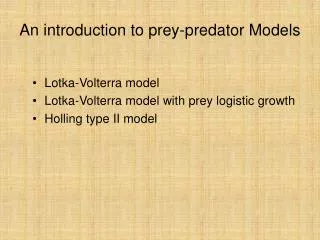
An introduction to prey-predator Models. Lotka-Volterra model Lotka-Volterra model with prey logistic growth Holling type II model. Generic Model. f(x) prey growth term g(y) predator mortality term h(x,y) predation term e prey into predator biomass conversion coefficient.

E N D
An introduction to prey-predator Models • Lotka-Volterra model • Lotka-Volterra model with prey logistic growth • Holling type II model
Generic Model • f(x) prey growth term • g(y) predator mortality term • h(x,y) predation term • e prey into predator biomass conversion coefficient
Lotka-Volterra Model • r prey growth rate : Malthus law • m predator mortality rate : natural mortality • Mass action law • a and b predation coefficients : b=ea • e prey into predator biomass conversion coefficient
Local stability analysis • Jacobian at positive equilibrium • detJ*>0 and trJ*=0 (center)
Local stability analysis • Proof of existence of center trajectories (linearization theorem) • Existence of a first integral H(x,y) :
Nullclines for the Lotka-Volterra model with prey logistic growth
Lotka-Volterra Model with prey logistic growth • Equilibrium points : (0,0) (K,0) (x*,y*)
Local stability analysis • Jacobian at positive equilibrium • detJ*>0 and trJ*<0 (stable)
Lotka-Volterra model with prey logistic growth : coexistence
Lotka-Volterra with prey logistic growth : predator extinction
Transcritical bifurcation (K,0) stable and (x*,y*) unstable and negative (K,0) and (x*,y*) same (K,0) unstable and (x*,y*) stable and positive
Loss of periodic solutions coexistence Predator extinction
Existence of limit cycle (Supercritical Hopf bifurcation) • Polar coordinates
Poincaré-Bendixson Theorem • A bounded semi-orbit in the plane tends to : • a stable equilibrium • a limit cycle • a cycle graph
Example of a trapping region • Van der Pol model (l>0)
Paradox of enrichment • When K increases : • Predator extinction • Prey-predator coexistence (TC) • Prey-predator equilibrium becomes unstable (Hopf) • Occurrence of a stable limit cycle (large variations)
Other prey-predator models • Functional responses (Type III, ratio-dependent …) • Prey-predator-super-predator… • Trophic levels
Routh-Hurwitz stability conditions • Characteristic equations • Stability conditions : M* l.a.s.
Routh-Hurwitz stability conditions • Dimension 2 • Dimension 3
Interspecific competition Model • Transformed system