History of Finite Element Analysis

1. History of Finite Element Analysis Finite Element Analysis (FEA) was first developed in 1943 by R. Courant, who utilized the Ritz method of numerical analysis and minimization of variational calculus. A paper published in 1956 by M. J. Turner, R. W. Clough, H. C. Martin, and L. J. Topp established a broader definition of numerical analysis. The paper centered on the "stiffness and deflection of complex structures". By the early 70's, FEA was limited to expensive mainframe computers generally owned by the aeronautics, automotive, defense, and nuclear industries. Since the rapid decline in the cost of computers and the phenomenal increase in computing power, FEA has been developed to an incredible precision. Mechanical Engineering Dept

2. Basics of Finite Element Analysis Why FEM ? • Modern mechanical design involves complicated shapes, sometimes made of different materials. • Engineers need to use FEM to evaluate their designs. Mechanical Engineering Dept

3. Basics of Finite Element Analysis FEA Applications • Evaluate the stress or temperature distribution in a mechanical component. • Perform deflection analysis. • Analyze the kinematics or dynamic response. • Perform vibration analysis. Mechanical Engineering Dept

4. Basics of Finite Element Analysis Consider a cantilever beam shown. Finite element analysis starts with an approximation of the region of interest into a number of meshes (triangular elements). Each mesh is connected to associated nodes (black dots) and thus becomes a finite element. Mechanical Engineering Dept

5. Basics of Finite Element Analysis • After approximating the object by finite elements, each node is associated with the unknowns to be solved. • For the cantilever beam the displacements in x and y would be the unknowns. • This implies that every node has two degrees of freedom and the solution process has to solve 2n degrees of freedom. • Once the displacements have been computed, the strains are derived by partial derivatives of the displacement function and then the stresses are computed from the strains. Mechanical Engineering Dept

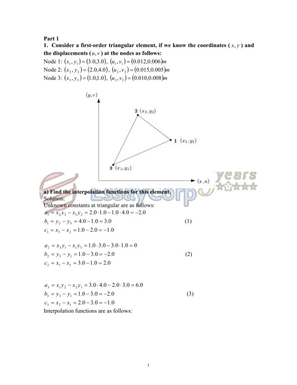
6. using two triangular elements, Example – a plate under load Py Derive and solve the system of equations for a plate loaded as shown. Plate thickness is 1 cm and the applied load Py is constant. Mechanical Engineering Dept

7. Example – a plate under load Displacement within the triangular element with three nodes can be assumed to be linear. u = α1 + α2 x + α3 y v = β1 + β2x + β3y Mechanical Engineering Dept

8. Example – a plate under load Displacement for each node, Mechanical Engineering Dept

9. Example – a plate under load Solve the equations simultaneously for α and β, Mechanical Engineering Dept

10. Calculations: 2a = 40 a1 = 40, a2 = 0, a3 = 0 b1 = - 4, b2 = 4, b3 = 0 c1 = -10, c2 = 0, c3 = 10 Example – a plate under load Substitute x1= 0, y1= 0, x2=10, y2= 0, x3= 0, y3=4 to obtain displacements u and v for element 1. (3) Element 1 (2) (1) Mechanical Engineering Dept

11. Change of notations u1 = U1, u2 = U3, u3 = U5, v1 = U2, v2 = U4, v3 = U6 2a = 40 a1 = 40, a2 = 0, a3 = 0 b1 = - 4, b2 = 4, b3 = 0 c1 = -10, c2 = 0, c3 = 10 β1 = (1)U2 β2 = -(1/10)U2 + (1/10) U4 β3 = -(1/4) U2+ (1/4) U6 Example Calculations: α1 = (1)U1 α2 = -(1/10)U1 + (1/10)U3 α3 = -(1/4) U1+ (1/4) U5 Mechanical Engineering Dept

12. Calculation: β1 = (1)U2 u1 = U1 + [-1/10(U1) + (1/10) U3] x + [-(1/4) U1+ (1/4) U5 ] y β2 = -(1/10)U2 + (1/10) U4 v1 = U2 + [-1/10(U2) + (1/10) U4] x + [-(1/4) U2+ (1/4) U6 ] y β3 = -(1/4) U2+ (1/4) U6 Example α1 = (1)U1 Substitute α and βto obtain displacements u and v for element 1. α2 = -(1/10)U1 + (1/10)U3 α3 = -(1/4) U1+ (1/4) U5 u = α1 + α2 x + α3 y v = β1 + β2x + β3y Mechanical Engineering Dept

13. Example u1 = U1 + [-1/10(U1) + (1/10) U3]x + [-(1/4) U1+ (1/4) U5 ] y v1= U2 + [-1/10(U2) + (1/10) U4]x + [-(1/4) U2+ (1/4) U6 ] y Rewriting the equations in the matrix form, Mechanical Engineering Dept

14. Example Similarly the displacements within element 2 can be expresses as Mechanical Engineering Dept

15. Example The next step is to determine the strains using 2D strain-displacement relations, Mechanical Engineering Dept

16. u1 = U1 + [-1/10(U1) + (1/10) U3] x + [-(1/4) U1+ (1/4) U5 ] y v1 = U2 + [-1/10(U2) + (1/10) U4] x + [-(1/4) U2+ (1/4) U6 ] y Example Differentiate the displacement equation to obtain the strain Mechanical Engineering Dept

17. Example Element 2 Mechanical Engineering Dept

18. We have: Example Using the stress-strain relations for homogeneous, isotropic material and plane-stress, εx = (σx / E ) - ν(εy) - ν(εz) = (σx / E ) - ν(σy / E ) - ν(σz / E ) εy = (σy / E ) - ν(εx) - ν(εz) = (σy / E ) - ν(σx / E ) - ν(σz / E ) εz = (σz / E ) - ν(εx) - ν(εy) = (σz / E ) - ν(σx / E ) - ν(σy / E ) Mechanical Engineering Dept

19. Formulation of the Finite Element Method • The classical finite element analysis code (h version) The system equations for solid and structural mechanics problems are derived using the principle of virtual displacement and work (Bathe, 1982). • The method of weighted residuals (Galerkin Method) weighted residuals are used as one method of finite element formulation starting from the governing differential equation. • Potential Energy and Equilibrium; The Rayleigh-Ritz Method. Involves the construction of assumed displacement field. Uses the total potential energy for an elastic body Mechanical Engineering Dept

20. f B – Body forces (forces distributed over the volume of the body: gravitational forces, inertia, or magnetic) f S – surface forces (pressure of one body on another, or hydrostatic pressure) f i – Concentrated external forces Formulation of the Finite Element Method Mechanical Engineering Dept

21. Let’s denote the displacements of any point (X, Y, Z) of the object from the unloaded configuration as UT The displacement U causes the strains and the corresponding stresses Formulation of the Finite Element Method The goal is to calculate displacement, strains, and stresses from the given external forces. Mechanical Engineering Dept

22. Formulation of the Finite Element Method Equilibrium condition and principle of virtual displacements The left side represents the internal virtual work done, and the right side represents the external work done by the actual forces as they go through the virtual displacement. The above equation is used to generate finite element equations. And by approximating the object as an assemblage of discrete finite elements, these elements are interconnected at nodal points. Mechanical Engineering Dept

23. Formulation of the Finite Element Method The equilibrium equation can be expressed using matrix notations for m elements. where B(m) Represents the rows of the strain displacement matrix C(m) Elasticity matrix of element m H(m) Displacement interpolation matrix U Vector of the three global displacement components at all nodes F Vector of the external concentrated forces applied to the nodes Mechanical Engineering Dept

24. Formulation of the Finite Element Method The above equation can be rewritten as follows, The above equation describes the static equilibrium problem. K is the stiffness matrix. Mechanical Engineering Dept

25. Continuing the example Mechanical Engineering Dept

26. Example Calculating the stiffness matrix for element 2. Mechanical Engineering Dept

27. Example The stiffness of the structure as a whole is obtained by combing the two matrices. Mechanical Engineering Dept

28. Example The load vector R, equals Rc because only concentrated loads act on the nodes. R = K = UR where Py is the known external force and F1x, F1y, F3x, and F3y are the unknown reaction forces at the supports. Mechanical Engineering Dept

29. Example The following matrix equation can be solved for nodal point displacements K = UR Mechanical Engineering Dept

30. The solution can be obtained by applying the boundary conditions Example Mechanical Engineering Dept

31. The equation can be divided into two parts, Example The first equation can be solved for the unknown nodal displacements, U3, U4, U7, and U8. And substituting these values into the second equation to obtain unknown reaction forces, F1x, F1y, F3x, and F3y . Once the nodal displacements have been obtained, the strains and stresses can be calculated. Mechanical Engineering Dept

32. Finite Element Analysis FEA is a mathematical representation of a physical system and the solution of that mathematical representation • Pre-Processing • Solving Matrix (solver) • Post-Processing FEA requires three steps Mechanical Engineering Dept

33. FEA Pre-Processing Mesh Mesh is your way of communicating geometry to the solver, the accuracy of the solution is primarily dependent on the quality of the mesh. The better the mesh looks, the more accurate the solution is. A good-looking mesh should have well-shaped elements, and the transition between densities should be smooth and gradual without skinny, distorted elements. Mechanical Engineering Dept

34. FEA Pre-Processing - meshing The mesh transition from .05 to .5 element size without control of transition (a) creates irregular mesh around the hole which will yield disappointing results. Mechanical Engineering Dept

35. FEA Pre-Processing Finite elements supported by most finite-element codes: Mechanical Engineering Dept

36. FEA Pre-Processing – Elements Beam Elements Beam elements typically fall into two categories; able to transmit moments or not able to transmit moments. Rod (bar or truss) elements cannot carry moments. Entire length of a modeled component can be captured with a single element. This member can transmit axial loads only and can be defined simply by a material and cross sectional area. Mechanical Engineering Dept

37. FEA Pre-Processing – Elements The most general line element is a beam. (a) and (b) are higher order line elements. Mechanical Engineering Dept

38. FEA Pre-Processing – Elements Plate and Shell Modeling Plate and shell are used interchangeably and refer to surface-like elements used to represent thin-walled structures. A quadrilateral mesh is usually more accurate than a mesh of similar density based on triangles. Triangles are acceptable in regions of gradual transitions. Mechanical Engineering Dept

39. Tetrahedral (tet) mesh is the only generally accepted means to fill a volume, used as auto-mesh by many FEA codes. 10-node Quadratic FEA Pre-Processing – Elements Solid Element Modeling Mechanical Engineering Dept

40. CAD Modeling for FEA CAD and FEA activities should be coordinated at the early stages of the design process to minimize the duplication of effort. • CAD models prepared by the design group for eventual FEA. • CAD models prepared without consideration of FEA needs. • CAD models unsuitable for use in analysis due to the amount of rework required. • Analytical geometry developed by or for analyst for sole purpose of FEA. Mechanical Engineering Dept

41. CAD Modeling for FEA • Solid chunky parts (thick-walled, low aspect ratio) parts mesh cleanly directly off CAD models. • Clean geometry geometrical features must not prevent the mesh from being created. The model should not include buried features. • Parent-child relationships parametric modeling allows defining features off other CAD features. Mechanical Engineering Dept

42. CAD Modeling for FEA Short edges and Sliver surfaces Short edges and sliver surfaces usually accompany each other and on large faces can cause highly distorted elements or a failed mesh. Mechanical Engineering Dept

43. CAD Modeling for FEA – Sliver Surfaces The rounded rib on the inside of the piston has a thickness of .30 and a radius of .145, as a result a flat surface of .01 by 2.5 is created. A mesh size of .05 is required to avoid distortedelements. This results in a 290,000 nodes. If the radius is increased to .15, a mesh size of .12 is sufficient which results in 33,500 nodes. Flat surface Mechanical Engineering Dept

44. CAD Modeling for FEA Sliver surface caused by misaligned features. Fillet across shallow angle Sliver surface caused by a slightly undersized fillet Mechanical Engineering Dept

45. Guidelines for Geometry Planning • Delay inclusion of fillets and chamfers as long as possible. • Try to use permanent datums as references where possible to minimize dependencies. • Avoid using fillet or draft edges as references for other features (parent-child relationship) • Never bury a feature in your model. Delete or redefine unwanted or incorrect features. Mechanical Engineering Dept

46. Guidelines for Part Simplification In general, features listed below could be considered for suppression. But, consider the impact before suppression. • Outside corner breaks or rounds. • Small inside fillets far from areas of interest. • Screw threads or spline features unless they are specifically being studied. • Small holes outside the load path. • Decorative or identification features. • Large sections of geometry that are essentially decoupled from the behavior of interested section. Mechanical Engineering Dept

47. Fillet added to the rib Holes removed Fillet removed Ribs needed for casting removed Guidelines for Part Simplification Mechanical Engineering Dept

48. CAD Modeling for FEAModel Conversion • Try to use the same CAD system for all components in design. • When the above is not possible, translate geometry through kernel based tools such as ACIS or Parasolids. Using standards based (IGES, DXF, or VDA) translations may lead to problem. • Visually inspect the quality of imported geometry. • Avoid modification of the imported geometry in a second CAD system. • Use the original geometry for analysis. If not possible, use a translation directly from the original model. Mechanical Engineering Dept

49. Example of a solid model corrupted by IGES transfer Mechanical Engineering Dept

50. FEA Pre-Processing Material Properties The only material properties that are generally required by an isotropic, linear static FEA are: Young’s modulus (E), Poisson’s ratio (v), and shear modulus (G). G = E / 2(1+v) Provide only two of the three properties. Thermal expansion and simulation analysis require coefficient of thermal expansion, conductivity and specific heat values. Mechanical Engineering Dept