Inventory Management Chapter 12
Inventory Management Chapter 12. © Prentice Hall 2007. General Considerations. Marketing-prefer large quantities of inventory Accounting/Finance-tied up capital Operations-tool that can be used to promote efficient operation of the production facilities

Inventory Management Chapter 12
E N D
Presentation Transcript
Inventory Management Chapter 12 © Prentice Hall 2007
General Considerations • Marketing-prefer large quantities of inventory • Accounting/Finance-tied up capital • Operations-tool that can be used to promote efficient operation of the production facilities • Inventories are simply allowed to fluctuate so that production can be adjusted to its most efficient level.
Types of Inventory • Pipeline Inventories: exist because materials must be moved from one location to another. • Buffer Inventories (safety stocks): provide protection against irregularities or uncertainties in an item’s demand or supply. • Anticipation Inventories: needed for products with seasonal patterns of demand and uniform supply.
Types of Inventory • Cycle Inventories (Lot-size inventories): exists whenever orders are made in larger quantities than needed to satisfy immediate requirements. Results from ordering in batches or “lots” rather than as needed.
Forms of Inventories • Raw Materials: objects, commodities, elements, and items that are received (usually purchased) from outside the organization to be used directly in the production of the final output. • Maintenance, repair, and operating supplies: used to support and maintain the operation, including spares, supplies, and stores.
Forms of Inventories • Work-In-Process (WIP): all the materials, parts, and assemblies that are being worked on or are waiting to be processed within the operations system. • Finished Goods: stock of completed products.
Placement of Inventories • Standard: An item is made to stock or ordered to stock and normally the item is available upon request. • Special: An item made to order.
Inventory-Related Costs • Ordering or Setup Costs: ordering costs are associated with outside procurement of material and setup costs are costs associated with internal procurement (i.e. internal manufacture) of parts of material. Ex: writing the order, processing the order through the purchasing system, postage, processing invoices, handling, testing, inspection, transportation, setup labor, machine downtime due to a new setup, parts damaged during setup. • Inventory Carrying or Holding Costs: cost items related to inventory quantity, items’ value, and length of the time the inventory is carried. Ex: interest on money invested in inventory and in the land, buildings, and equipment necessary to hold and maintain the inventory; heat, power, and light, salaries of security personnel, taxes and insurance on equipment; insurance on inventory, physical deterioration of the inventory.
Inventory-Related Costs • Stockout Costs: if inventory is unavailable when customers request it, a situation that marketing detests, or when it is needed for production, a stockout occurs. Ex: lost goodwill, lost sales, cost associated with processing back orders (such as extra paperwork, special handling, and higher shipping costs)
Determining inventory system performance • Inventory turnover: relates inventory levels to the products sales volume. • Turnover is often used to compare an individual firm’s performance with others in the same industry or to monitor the effects of a change in inventory decision rules.
Example of measuring inventory system performance Suppose a company’s new annual report claims their costs of goods sold for the year is $160 million and their total average inventory (production materials + work-in-process) is worth $35 million. This company normally has an inventory turn ratio of 10. What is this year’s Inventory Turnover ratio? What does it mean?
Example of measuring inventory system performance(Continued) = $160/$35 = 4.57 Since the company’s normal inventory turnover ratio is 10, a drop to 4.57 means that the inventory is not turning over as quickly as it had in the past. Without knowing the industry average of turns for this company it is not possible to comment on how they are competitively doing in the industry, but they now have more inventory relative to their cost of goods sold than before.
Determining inventory system performance • Fill rate: to capture the benefits of having inventory, some companies use customer service to asses their inventory system performance. • The percentage of units immediately available when requested by customers.
Priorities for Inventory Management: The ABC Analysis • Classifying inventory according to some measure of importance and allocating control efforts accordingly. • A items • 15-20% of items that account for 75-80% of annual inventory value, should be subject to the tightest control. • B items • 30-40% of items that account for 15% of annual inventory value • C items • 40-50% of items that account for 10-15% of annual inventory value
Assumptions Economic Order Quantity Demand rate is constant No constraints on lot size Only relevant costs are holding and ordering/setup Decisions for items are independent from other items No uncertainty in lead time or supply
When to use EOQ • Don’t use; if you use the “make-to-order” strategy • Modify it; if significant quantity discounts are given for ordering larger lots • Use it; if you follow a “make-to-stock” strategy (stable demand)
Receive order Inventory depletion (demand rate) Q On-hand inventory (units) Average cycle inventory Q — 2 1 cycle Time Economic Order Quantity
Total cost = HC + OC Annual cost (dollars) Holding cost (HC) Ordering cost (OC) Lot Size (Q) Economic Order Quantity
3000 — 2000 — 1000 — 0 — Q 2 D Q Total cost = (H) + (S) Q 2 Annual cost (dollars) Holding cost = (H) D Q Ordering cost = (S) | | | | | | | | 50 100 150 200 250 300 350 400 Lot Size (Q) Economic Order Quantity
Annual carrying cost Annual ordering cost Total cost = + Q D S H TC = + 2 Q Basic Economic-Order Quantity (EOQ) Model Formula TC=Total annual cost D =Demand C =Cost per unit Q =Order quantity S =Cost of placing an order or setup cost R =Reorder point L =Lead time H=Annual holding and storage cost per unit of inventory
3000 — 2000 — 1000 — 0 — Q 2 D Q Total cost = (H) + (S) Q 2 Annual cost (dollars) Holding cost = (H) D = (18 /week)(52 weeks) = 936 units H = 0.25 ($60/unit) = $15 S = $45 Q = 390 units D Q Q 2 D Q Ordering cost = (S) C = (H) + (S) | | | | | | | | 50 100 150 200 250 300 350 400 Lot Size (Q) Economic Order Quantity Bird feeder costs C = $2925 + $108 = $3033
Current cost 3000 — 2000 — 1000 — 0 — Q 2 D Q Total cost = (H) + (S) Bird feeder costs Q 2 Annual cost (dollars) Holding cost = (H) D = (18 /week)(52 weeks) = 936 units H = 0.25 ($60/unit) = $15 S = $45 Q = 390 units D Q Q 2 D Q Ordering cost = (S) C = (H) + (S) | | | | | | | | 50 100 150 200 250 300 350 400 C = $2925 + $108 = $3033 Current Q Lot Size (Q) Economic Order Quantity
Current cost 3000 — 2000 — 1000 — 0 — Q 2 D Q Total cost = (H) + (S) Bird feeder costs Q 2 Annual cost (dollars) Holding cost = (H) D = (18 /week)(52 weeks) = 936 units H = 0.25 ($60/unit) = $15 S = $45 Q = 468 units D Q Q 2 D Q Ordering cost = (S) C = (H) + (S) | | | | | | | | 50 100 150 200 250 300 350 400 Current Q Lot Size (Q) Economic Order Quantity C = $3510 + $90 = $3600
Current cost 3000 — 2000 — 1000 — 0 — Q 2 D Q D = (18 /week)(52 weeks) = 936 units H = 0.25 ($60/unit) = $15 S = $45 Q = EOQ Total cost = (H) + (S) Q 2 Annual cost (dollars) Holding cost = (H) Q 2 D Q 2DS H C = (H) + (S) EOQ = D Q Ordering cost = (S) | | | | | | | | 50 100 150 200 250 300 350 400 Current Q Lot Size (Q) Economic Order Quantity Bird feeder costs
Current cost 3000 — 2000 — 1000 — 0 — Q 2 D Q D = (18 /week)(52 weeks) = 936 units H = 0.25 ($60/unit) = $15 S = $45 Q = 75 Total cost = (H) + (S) Q 2 Annual cost (dollars) Holding cost = (H) Q 2 D Q 2DS H C = (H) + (S) EOQ = D Q Ordering cost = (S) | | | | | | | | 50 100 150 200 250 300 350 400 Current Q Lot Size (Q) Economic Order Quantity Bird feeder costs
Current cost 3000 — 2000 — 1000 — 0 — Q 2 D Q D = (18 /week)(52 weeks) = 936 units H = 0.25 ($60/unit) = $15 S = $45 Q = 75 Total cost = (H) + (S) Q 2 Annual cost (dollars) Holding cost = (H) Q 2 D Q 2DS H C = (H) + (S) EOQ = C = $562 + $562 = $1124 D Q Ordering cost = (S) | | | | | | | | 50 100 150 200 250 300 350 400 Current Q Lot Size (Q) Economic Order Quantity Bird feeder costs
Current cost 3000 — 2000 — 1000 — 0 — Bird feeder costs Q 2 D Q D = (18 /week)(52 weeks) = 936 units H = 0.25 ($60/unit) = $15 S = $45 Q = 75 Total cost = (H) + (S) Q 2 Annual cost (dollars) Holding cost = (H) Q 2 D Q 2DS H C = (H) + (S) EOQ = C = $562 + $562 = $1124 D Q Ordering cost = (S) Lowest cost | | | | | | | | 50 100 150 200 250 300 350 400 Current Q Best Q (EOQ) Lot Size (Q) Economic Order Quantity
Current cost 3000 — 2000 — 1000 — 0 — Bird feeder costs Q 2 D Q D = (18 /week)(52 weeks) = 936 units H = 0.25 ($60/unit) = $15 S = $45 Q = 75 Total cost = (H) + (S) Q 2 Annual cost (dollars) Holding cost = (H) Q 2 D Q 2DS H C = (H) + (S) EOQ = C = $562 + $562 = $1124 D Q Ordering cost = (S) Lowest cost | | | | | | | | 50 100 150 200 250 300 350 400 Current Q Best Q (EOQ) Lot Size (Q) Economic Order Quantity
Current cost 3000 — 2000 — 1000 — 0 — Bird feeder costs Q 2 D Q D = (18 /week)(52 weeks) = 936 units H = 0.25 ($60/unit) = $15 S = $45 Q = 75 Total cost = (H) + (S) EOQ D TBOEOQ = = 75/936 = 0.080 year Q 2 Annual cost (dollars) Holding cost = (H) Q 2 D Q 2DS H C = (H) + (S) EOQ = C = $562 + $562 = $1124 D Q Ordering cost = (S) Lowest cost | | | | | | | | 50 100 150 200 250 300 350 400 Current Q Best Q (EOQ) Lot Size (Q) Economic Order Quantity Time between orders TBOEOQ = (75/936)(12) = 0.96 months TBOEOQ = (75/936)(52) = 4.17 weeks TBOEOQ = (75/936)(365) = 29.25 days
EOQ Example (1) Problem Data Given the information below, what are the EOQ and reorder point? Annual Demand = 1,000 units Days per year considered in average daily demand = 365 Cost to place an order = $10 Holding cost per unit per year = $2.50 Lead time = 7 days Cost per unit = $15
EOQ Example (1) Solution In summary, you place an optimal order of 90 units. In the course of using the units to meet demand, when you only have 20 units left, place the next order of 90 units.
EOQ Example (2) • Given: • 25,000 annual demand • $3 per unit per year holding cost • $100 ordering costs
Independent Demand (Demand for the final end-product or demand not related to other items) Dependent Demand (Derived demand items for component parts, subassemblies, raw materials, etc) Independent vs. Dependent Demand Finished product E(1) Component parts
Decisions in Inventory Management Only two decisions need to be made in managing independent-demand inventories: • When to order? (timing) • How much to order? (size)
Routine inventory decisions • These two decisions can be made routinely by using any one of four inventory control decision rules in figure below: Q, order a fixed quantity Q S, order up to a fixed expected opening inventory quantity S R, place an order when the inventory balance drops to R T, place an order every T periods
How Much? When!
Types of Inventory Management Systems • Continuous review (Reorder point) systems • time between orders varies • constant order quantity • Periodic review systems • time between orders fixed • order quantity varies • Material requirements planning (MRP) • dependent demand items
Continuous Review (Reorder point system) • Reorder point: whenever the inventory on hand reaches the predetermined inventory level-thereorder point- an order may be placed for a prespecified amount if there are no current outstanding orders. • Order quantity is fixed, and the reorder period varies. • Lead time: the time between placement of an order and receipt of the shipment. • The quantity of inventory to be ordered is often based on economic order quantity (one answer to the question “how much to order”). It can be also based on a price-break quantity, or a container size (such as a truckload).
Continuous Review Systems • Two-bin system: much-used variation of the reorder point system. Parts are stored in two bins-one large and one small. • Small bin- holds sufficient parts to satisfy the demand. • Large bin- parts are used from only the large bin, until it is empty. • Advantage-inventory need not be continually recounted to determine whether or not a reorder should be placed.
Continuous Review Systems • Perpetual inventory system: System that keeps track of removals from inventory continuously, thus monitoring current levels of each item. • Requires either a manual card system or a computerized system to keep track of daily usage and daily stock levels. • A reorder point system could not adequately perform without either a two-bin system or perpetual inventory system.
Continuous Review Systems • Continuous review system tracks the remaining inventory of an item each time a withdrawal is made to determine whether it is time to reorder. • At each review, a decision is made about an item’s inventory position (IP). • Inventory position (IP)=On-hand inventory (OH)+ scheduled receipts (open orders) (SR)-backorders (BO)
Soup Soup Soup IP IP IP Order received Order received Order received Order received Q Q Q On-hand inventory OH OH OH R Order placed Order placed Order placed Time L L L TBO TBO TBO Continuous Review (Reorder point system)
Example • Demand for chicken soup at a supermarket is always 25 cases a day and the lead time is always four days. The shelves were just restocked with chicken soup, leaving an on-hand inventory of only 10 cases. There are no backorders, but there is one open order for 200 cases. What is the inventory position? Should a new order be placed?
Soup Soup Soup IP IP IP Order received Order received Order received Order received Chicken Soup Q Q Q On-hand inventory R = Average demand during lead time = (25)(4) = 100 cases IP = OH + SR – BO = 10 + 200 – 0 = 210 cases OH OH OH R Order placed Order placed Order placed Time L L L TBO TBO TBO Continuous Review
IP IP Order received Order received Order received Order received Q Q Q OH On-hand inventory R Order placed Order placed Order placed Time L1 L2 L3 TBO1 TBO2 TBO3 Uncertain Demand
Reorder Point / Safety Stock • Because of uncertain demand, sales during lead time are unpredictable, and safety stock is added to hedge against lost sales. • Deciding on a small or large safety stock is a trade-off between customer service and inventory holding costs. • The usual approach for determining R is for management is to set a reasonable service level policy for the inventory and then determine the safety stock level that satisfies this policy. • Service level is the desired probability of not running out of stock in any one ordering cycle, which begins at the time an order is placed and ends when it arrives in stock.
Cycle-service level = 85% Probability of stockout (1.0 – 0.85 = 0.15) Average demand during lead time Average demand during lead time R zL z=the number of standard deviations for a specified service probability σL=standard deviation of demand during lead time Reorder Point / Safety Stock
Example • Records show that the demand for dishwasher detergent during lead time is normally distributed, with an average of 250 boxes and σL=22. What safety stock should be carried for a 99 percent cycle-service level? What is R?