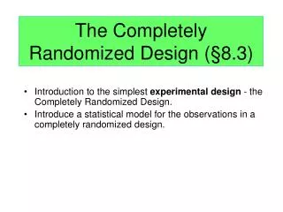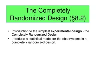
Completely Randomized Design
Completely Randomized Design. Completely Randomized Design. 1. Experimental Units (Subjects) Are Assigned Randomly to Treatments Subjects are Assumed Homogeneous 2. One Factor or Independent Variable 2 or More Treatment Levels or Classifications 3. Analyzed by One-Way ANOVA.


Completely Randomized Design
E N D
Presentation Transcript
Completely Randomized Design 1. Experimental Units (Subjects) Are Assigned Randomly to Treatments • Subjects are Assumed Homogeneous 2. One Factor or Independent Variable • 2 or More Treatment Levels or Classifications 3. Analyzed by One-Way ANOVA
Randomized Design Example
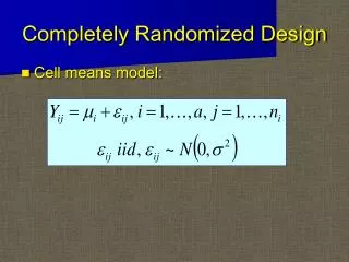
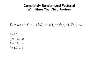
Xij =μ + ti+εij The Linier Model i = 1,2,…, t j = 1,2,…, r Xij = the observation inith treatment and thejth replication m = overall mean t i= the effect of theithtreatment eij = random error
One-Way ANOVA F-Test 1. Tests the Equality of 2 or More (t) Population Means 2. Variables • One Nominal Scaled Independent Variable • 2 or More (t) Treatment Levels or Classifications • One Interval or Ratio Scaled Dependent Variable 3. Used to Analyze Completely Randomized Experimental Designs
Assumptions 1. Randomness & Independence of Errors • Independent Random Samples are Drawn for each condition 2. Normality • Populations (for each condition) are Normally Distributed 3. Homogeneity of Variance • Populations (for each condition) have Equal Variances
Hypotheses • H0: 1 = 2 = 3 = ... = t • All Population Means are Equal • No Treatment Effect • Ha: Not All i Are Equal • At Least 1 Pop. Mean is Different • Treatment Effect NOT 12 ... t
Hypotheses • H0: 1 = 2 = 3 = ... = t • All Population Means are Equal • No Treatment Effect • Ha: Not All i Are Equal • At Least 1 Pop. Mean is Different • Treatment Effect NOT 12 ... t f(X) X = = 1 2 3 f(X) X = 1 2 3
One-Way ANOVA Basic Idea 1. Compares 2 Types of Variation to Test Equality of Means 2. Comparison Basis Is Ratio of Variances 3. If Treatment Variation Is Significantly Greater Than Random Variation then Means Are Not Equal 4. Variation Measures Are Obtained by ‘Partitioning’ Total Variation
One-Way ANOVA Partitions Total Variation Total variation
One-Way ANOVA Partitions Total Variation Total variation Variation due to treatment
One-Way ANOVAPartitions Total Variation Total variation Variation due to treatment Variation due to random sampling
Sum of Squares Among Sum of Squares Between Sum of Squares Treatment Among Groups Variation One-Way ANOVAPartitions Total Variation Total variation Variation due to treatment Variation due to random sampling
Sum of Squares Within Sum of Squares Error (SSE) Within Groups Variation Sum of Squares Among Sum of Squares Between Sum of Squares Treatment (SST) Among Groups Variation One-Way ANOVAPartitions Total Variation Total variation Variation due to treatment Variation due to random sampling
Total Variation Response, X X Group 1 Group 2 Group 3
Treatment Variation Response, X X3 X X2 X1 Group 1 Group 2 Group 3
Random (Error) Variation Response, X X3 X2 X1 Group 1 Group 2 Group 3
One-Way ANOVA F-Test Test Statistic 1. Test Statistic • F = MST / MSE • MST Is Mean Square for Treatment • MSE Is Mean Square for Error 2. Degrees of Freedom • 1 = t -1 • 2 = tr - t • t = # Populations, Groups, or Levels • tr = Total Sample Size
One-Way ANOVA Summary Table Source of Degrees Sum of Mean F Variation of Squares Square Freedom (Variance) Treatment t - 1 SST MST = MST SST/(t - 1) MSE Error tr - t SSE MSE = SSE/(tr - t) Total tr - 1 SS(Total) = SST+SSE
ANOVA Table for aCompletely Randomized Design Source of Sum of Degrees of Mean Variation Squares Freedom Squares F TreatmentsSST t - 1 SST/t-1 MST/MSE ErrorSSE tr- t SSE/tr-t TotalSSTot tr - 1
The F distribution • Two parameters • increasing either one decreases F-alpha (except for v2<3) • I.e., the distribution gets smashed to the left F 0 F ( v1 , v2 )
One-Way ANOVA F-Test Critical Value If means are equal, F = MST / MSE1. Only reject large F! Reject H 0 Do Not Reject H 0 F 0 F a ( t 1 , tr -t) Always One-Tail! © 1984-1994 T/Maker Co.
Example: Home Products, Inc. • Completely Randomized Design Home Products, Inc. is considering marketing a long-lasting car wax. Three different waxes (Type 1, Type 2, and Type 3) have been developed. In order to test the durability of these waxes, 5 new cars were waxed with Type 1, 5 with Type 2, and 5 with Type 3. Each car was then repeatedly run through an automatic carwash until the wax coating showed signs of deterioration. The number of times each car went through the carwash is shown on the next slide. Home Products, Inc. must decide which wax to market. Are the three waxes equally effective?
Example: Home Products, Inc. Wax Wax Wax Observation Type 1 Type 2 Type 3 1 27 33 29 2 30 28 28 3 29 31 30 4 28 30 32 5 31 30 31 Sample Mean 29.0 30.4 30.0 Sample Variance2.5 3.3 2.5
Example: Home Products, Inc. • Hypotheses H0: 1=2=3 Ha: Not all the means are equal where: 1 = mean number of washes for Type 1 wax 2 = mean number of washes for Type 2 wax 3 = mean number of washes for Type 3 wax
Example: Home Products, Inc. • Mean Square Between Treatments Since the sample sizes are all equal: μ= (x1 + x2 + x3)/3 = (29 + 30.4 + 30)/3 = 29.8 SSTR= 5(29–29.8)2+ 5(30.4–29.8)2+ 5(30–29.8)2= 5.2 MSTR = 5.2/(3 - 1) = 2.6 • Mean Square Error SSE = 4(2.5) + 4(3.3) + 4(2.5) = 33.2 MSE = 33.2/(15 - 3) = 2.77 _ _ _ =
Example: Home Products, Inc. • Rejection Rule Using test statistic: Reject H0 if F > 3.89 Using p-value: Reject H0 if p-value < .05 where F.05 = 3.89 is based on an F distribution with 2 numerator degrees of freedom and 12 denominator degrees of freedom
Example: Home Products, Inc. • Test Statistic F = MST/MSE = 2.6/2.77 = .939 • Conclusion Since F = .939 < F.05 = 3.89, we cannot reject H0. There is insufficient evidence to conclude that the mean number of washes for the three wax types are not all the same.
Example: Home Products, Inc. • ANOVA Table Source of Sum of Degrees of Mean Variation Squares Freedom Squares F Treatments5.2 2 2.60 .9398 Error 33.2 12 2.77 Total38.4 14
Using Excel’s ANOVA: Single Factor Tool • Value Worksheet (top portion)
Using Excel’s ANOVA: Single Factor Tool • Value Worksheet (bottom portion)
Using Excel’s ANOVA: Single Factor Tool • Conclusion Using the p-Value • The value worksheet shows a p-value of .418 • The rejection rule is “Reject H0 if p-value < .05” • Because .418 > .05, we cannot reject H0. There is insufficient evidence to conclude that the mean number of washes for the three wax types are not all the same.
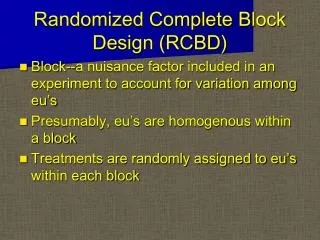
RCBD (Randomized Complete Block Design)
Randomized Complete Block Design • An experimental design in which there is one independent variable, and a second variable known as a blocking variable, that is used to control for confounding or concomitant variables. • It is used when the experimental unit or material are heterogeneous • There is a way to block the experimental units or materials to keep the variability among within a block as small as possible and to maximize differences among block • The block (group) should consists units or materials which are as uniform as possible
Randomized Complete Block Design • Confounding or concomitant variable are not being controlled by the analyst but can have an effect on the outcome of the treatment being studied • Blocking variable is a variable that the analyst wants to control but is not the treatment variable of interest. • Repeated measures designis a randomized block design in which each block level is an individual item or person, and that person or item is measured across all treatments.
The Blocking Principle • Blocking is a technique for dealing with nuisancefactors • A nuisance factor is a factor that probably has some effect on the response, but it is of no interest to the experimenter…however, the variability it transmits to the response needs to be minimized • Typical nuisance factors include batches of raw material, operators, pieces of test equipment, time (shifts, days, etc.), different experimental units • Many industrial experiments involve blocking (or should) • Failure to block is a common flaw in designing an experiment
The Blocking Principle • If the nuisance variable is known and controllable, we use blocking • If the nuisance factor is known and uncontrollable, sometimes we can use the analysis of covariance to statistically remove the effect of the nuisance factor from the analysis • If the nuisance factor is unknown and uncontrollable (a “lurking” variable), we hope that randomization balances out its impact across the experiment • Sometimes several sources of variability are combined in a block, so the block becomes an aggregate variable
Partitioning the Total Sum of Squares in the Randomized Block Design SStotal (total sum of squares) SSE (error sum of squares) SST (treatment sum of squares) SSB (sum of squares blocks) SSE’ (sum of squares error)
Single Independent Variable Blocking Variable . Individual observations . . . . . . . . . . . . . . . . A Randomized Block Design
The Linier Model i = 1,2,…, t j = 1,2,…,r yij = the observation inith treatment in thejth block m = overall mean ti = the effect of theithtreatment No interaction between blocks and treatments rj = the effect of the jth block eij = random error
Extension of the ANOVA to the RCBD ANOVA partitioning of total variability:
Extension of the ANOVA to the RCBD The degrees of freedom for the sums of squares in are as follows: • Ratios of sums of squares to their degrees of freedom result in mean squares, and • The ratio of the mean square for treatments to the error mean square is an F statistic used to test the hypothesis of equal treatment means
ANOVA Procedure • The ANOVA procedure for the randomized block design requires us to partition the sum of squares total (SST) into three groups: sum of squares due to treatments, sum of squares due to blocks, and sum of squares due to error. • The formula for this partitioning is SSTot = SSTreatment + SSBlock + SSE • The total degrees of freedom, tr - 1, are partitioned such that t - 1 degrees of freedom go to treatments, r - 1 go to blocks, and (t - 1)(r - 1) go to the error term.
ANOVA Table for aRandomized Block Design Source of Sum of Degrees of Mean Variation Squares Freedom Squares F TreatmentsSST t – 1 SST/t-1 MST/MSE BlocksSSB r - 1 ErrorSSE (t - 1)(r - 1) SSE/(t-1)(r-1) TotalSSTot tr - 1
Example: Eastern Oil Co. Randomized Block Design Eastern Oil has developed three new blends of gasoline and must decide which blend or blends to produce and distribute. A study of the miles per gallon ratings of the three blends is being conducted to determine if the mean ratings are the same for the three blends. Five automobiles have been tested using each of the three gasoline blends and the miles per gallon ratings are shown on the next slide.
Example: Eastern Oil Co. Automobile Type of Gasoline (Treatment) Blocks (Block)Blend XBlend YBlend Z Means 1 32 31 30 31 2 29 28 27 28 3 30 30 27 29 4 32 31 30 31 5 27 25 26 26 Treatment Means 30 29 28 29