III. Completely Randomized Design (CRD)
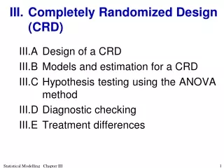
III. Completely Randomized Design (CRD). III.A Design of a CRD III.B Models and estimation for a CRD III.C Hypothesis testing using the ANOVA method III.D Diagnostic checking III.E Treatment differences. III.A Design of a CRD.

III. Completely Randomized Design (CRD)
E N D
Presentation Transcript
III. Completely Randomized Design (CRD) III.A Design of a CRD III.B Models and estimation for a CRD III.C Hypothesis testing using the ANOVA method III.D Diagnostic checking III.E Treatment differences Statistical Modelling Chapter III
III.A Design of a CRD Definition III.1: An experiment is set up using a CRD when each treatment is applied a specified, possibly unequal, number of times, the particular units to receive a treatment being selected completely at random. Example III.1 Rat experiment • Experiment to investigate 3 rat diets with 6 rats: Diet A, B, C will have 3, 2, 1 rats, respectively. Statistical Modelling Chapter III
Use R to obtain randomized layouts • How to do this is described in Appendix B, Randomized layouts and sample size computations in , for all the designs that will be covered in this course, and more besides. Statistical Modelling Chapter III
R functions and output to produce randomized layout > # Obtaining randomized layout for a CRD > # > n <- 6 > CRDRat.unit <- list(Rat = n) > Diet <- factor(rep(c("A","B","C"), > times = c(3,2,1))) > CRDRat.lay <- fac.layout(unrandomized=CRDRat.unit, > randomized=Diet, seed=695) > CRDRat.lay • fac.layout from dae package produces the randomized layout. • unrandomized gives the single unrandomized factor indexing the units in the experiment. • randomized specifies the factor, Diets, that is to be randomized. • seed is used so that the same randomized layout for a particular experiment can be generated at a later date. (0–1023) Statistical Modelling Chapter III
Randomized layout Units Permutation Rat Diet 1 1 4 1 A 2 2 1 2 C 3 3 5 3 B 4 4 3 4 A 5 5 6 5 A 6 6 2 6 B #remove Diet object in workspace to avoid using it by mistake remove(Diet) Statistical Modelling Chapter III
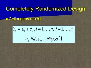
III.B Models and estimation for a CRD • The analysis of CRD experiments uses: • least-squares or maximum likelihood estimation of the parameters of a linear model • hypothesis testing based on the ANOVA method or maximum likelihood ratio testing. • Use rat experiment to investigate linear models and the estimation of its parameters. Statistical Modelling Chapter III
a) Maximal model • Definition III.2: The maximal expectation model is the most complicated model for the expectation that is to be considered in analysing an experiment. • We first consider the maximal model for the CRD. Statistical Modelling Chapter III
Our model also involves assuming Example III.1 Rat experiment (continued) • Suppose, the experimenter measured the liver weight as a percentage of total body weight at the end of the experiment. • The results of the experiment are as follows: • The analysis based on a linear model, that is: • Trick is what are X and q going to be? Statistical Modelling Chapter III
The fitted equation is: Perhaps? • Note numbering of Y's does not correspond to Rats; does not affect model but neater. • This model can then be fitted using simple linear regression techniques. Statistical Modelling Chapter III
Using model to predict • However, does this make sense? • means that, for each unit increase in diet, % liver weight decreases by 0.120. • sensible only if the diets differences are based on equally spaced levels of some component; • For example, if the diets represent 2, 4 and 6 mg of copper added to each 100g of food • But, no good if diets unequally spaced (2, 4, and 10 mg Cu added) or diets differ qualitatively. Statistical Modelling Chapter III
Regression on indicator variables • In this method the explanatory variables are called factors and the possible values they take levels. • Thus, we have a factor Diet with 3 levels: A, B, C. • Definition III.3: Indicator variables are formed from a factor: • create a variable for each level of the factor; • the values of a variable are either 1 or 0, 1 when the unit has the particular level for that variable and 0 otherwise. Statistical Modelling Chapter III
Indicator-variable model • Hence E[Yi] =ak, var[Yi] =s2, cov[Yi, Yj] = 0, (i j) • Can be written as • Model suggests 3 different expected (or mean) values for the diets. Statistical Modelling Chapter III
General form of X for CRD • For the general case of a set of t Treatments suppose Y is ordered so that all observations for: • 1st treatment occur in the first r1 rows, • 2nd treatment occur in the next r2 rows, • and so on with the last treatment occurring in the last rt rows. • i.e. order of systematic layout (prior to randomization) • Then XT given by the following partitioned matrix (1 only ever vector, but 0 can be matrix) Statistical Modelling Chapter III
Still a linear model • In general, the model for the expected values is still of the general form E[Y] = Xq • and on assuming Y is • can use standard least squares or maximum likelihood estimation Statistical Modelling Chapter III
Estimates of expectation parameters • Can be shown, by examining the OLS equation, that the estimates of the elements of a and y are the means of the treatments. • Example III.1 Rat experiment (continued) • OLS equation is • The estimates of a are: Statistical Modelling Chapter III
Example III.1 Rat experiment (continued) • The estimates of the expected values, the fitted values, are given by: Statistical Modelling Chapter III
Estimator of the expected values • In general, where is the n-vector consisting of the treatment means for each unit and • being least squares, this estimator can be written as a linear combination of Y. • that is, can be obtained as the product of an matrix and the n-vector Y. • let us write • M for mean because MT is the matrix that replaces each value of Y with the mean of the corresponding treatment. Statistical Modelling Chapter III
Clear from the above expression that: • 1str1 elements of are the mean of the Yis for the 1st treatment, • next r2 elements are the mean of those for the 2nd treatment, • and so on. General form of mean operator • Can be shown that the general form of MT is • MT is a mean operator as it • computes the treatment means from the vector to which it is applied and • replaces each element of this vector with its treatment mean. Statistical Modelling Chapter III
Estimator of the errors • The estimator of the random errors in the observed values of Y is, as before, the difference from the expected values. • That is, Statistical Modelling Chapter III
Example III.1 Rat experimentAlternative expression for fitted values • We know that where Note not as estimates rather than estimators. Statistical Modelling Chapter III
Residuals • Fitted values for orthogonal experiments are functions of means. • Residuals are differences between observations and fitted values Statistical Modelling Chapter III
b) Alternative indicator-variable, expectation models • For the CRD, two expectation models are considered: • First model is minimal expectation model: population mean response is same for all observations, irrespective of diet. • Second model is the maximal expectation model. Statistical Modelling Chapter III
Minimal expectation model • Definition III.4: The minimal expectation model is the simplest model for the expectation that is to be considered in analysing an experiment. • The minimal expectation model is the same as the intercept-only model given for the single sample in chapter I, Statistical inference. • Will be this for all analyses we consider. • Now the estimator of the expected values in the intercept-only model is where is the n-vector each of whose elements is the grand mean. • For Rat experiment Statistical Modelling Chapter III
Marginal models • In regression case obtained marginal models by zeroing some of the parameters in the full model. • Here this is not the case. • Instead impose equality constraints. • Here simply set ak = m • That is, intercept only model is the special case where all ak s are equal. • Clear for getting E[Yi] = m from E[Yi] = ak. • What about yG from yT? • If replace each element of a with m, then a = 1tm. • So yT = XTa = XT1tm = XGm. • Now marginality expressed in the relationship between XT and XG as encapsulated in definition. Statistical Modelling Chapter III
Marginality of models (in general) • Definition III.5: Let C(X) denote the column space of X. • For two models, y1 X1q1 and y2 X2q2, the first model is marginal to the second if C(X1) C(X2) irrespective of the replication of the levels in the columns of the Xs, • That is if the columns of X1 can always be written as linear combinations of the columns of X2. • We write y1 y2. • Note marginality relationship is not symmetric — it is directional, like the less-than relation. • So while y1 y2, y2 is not marginal to y1 unless y1 y2. Statistical Modelling Chapter III
Marginality of models for CRD • yG is marginal toyT or yG yT because C(XG) C(XT) • in that an element from a row of XG is the sum of the elements in the corresponding row of XT • and this will occur irrespective of the replication of the levels in the columns of XG and XT. • So while yG yT, yT is not marginal to yG as C(XT) C(XG) so that yTyG. • In geometrical terms, C(XT) is a three-dimensional space and C(XG) is a line, the equiangular line, that is a subspace of C(XT). Statistical Modelling Chapter III
III.C Hypothesis testing using the ANOVA method • Are there significant differences between the treatment means? • This is equivalent to deciding which of our two expectation models best describes the data. • We now perform the hypothesis test to do this for the example. Statistical Modelling Chapter III
Analysis of the rat exampleExample III.1 Rat experiment (continued) Step 1: Set up hypotheses H0: aA = aB = aC = m (yG XGm) H1: not all population Diet means are equal (yD XDa) Set a = 0.05 Statistical Modelling Chapter III
Example III.1 Rat experiment (continued) Step 2: Calculate test statistic • From table can see that (corrected) total variation amongst the 6 Rats is partitioned into 2 parts: • variance of difference between diet means and • the left-over (residual) rat variation. • Step 3: Decide between hypotheses • As probability of exceeding F of 3.60 with n1= 2 and n2= 3 is 0.1595 > a = 0.05, not much evidence of a diet difference. • Expectation model that appears to provide an adequate description of the data is yG XGm. Statistical Modelling Chapter III
b) Sums of squares for the analysis of variance • From chapter I, Statistical inference, an SSq • is the SSq of the elements of a vector and • can write as the product of transpose of a column vector with original column vector. • Estimators of SSqs for the CRD ANOVA are SSqs of following vectors (cf ch.I): where Ds are n-vectors of deviations from Y and Te is the n-vector of Treatment effects. Definition III.6: An effect is a linear combination of means with a set of effects summing to zero. Statistical Modelling Chapter III
SSqs as quadratic forms • Want to show estimators of all SSqs can be written as YQY. • Is product of 1n, nn and n1 vectors and matrix, so is 11 or a scalar. • Definition III.7: A quadratic form in a vector Y is a scalar function of Y of the form YAY where A is called the matrix of the quadratic form. Statistical Modelling Chapter III
SSqs as quadratic forms (continued) • Firstly write • That is, each of the individual vectors on which the sums of squares are based can be written as an M matrix times Y. • These M matrices are mean operators that are symmetric and idempotent: M'=M and M2=M in all cases. Statistical Modelling Chapter III
SSqs as quadratic forms (continued) • Then • Given Ms are symmetric and idempotent, it is relatively straightforward to show so are the three Q matrices. • It can also be shown that Statistical Modelling Chapter III
SSqs as quadratic forms (continued) • Consequently obtain the following expressions for the SSqs: Statistical Modelling Chapter III
SSqs as quadratic forms (continued) • Theorem III.1: For a completely randomized design, the sums of squares in the analysis of variance for Units, Treatments and Residual are given by the quadratic form: Proof: follows the argument given above. Statistical Modelling Chapter III
In the notes show that • so that Residual SSq by difference • That is, Residual SSq = Units SSq - Treatments SSq. Statistical Modelling Chapter III
ANOVA table construction • As in regression, Qs are orthogonal projection matrices. • QU orthogonally projects the data vector into the n-1 dimensional part of the n-dimensional data space that is orthogonal to equiangular line. • QT orthogonally projects data vector into the t-1 dimensional part of the t-dimensional Treatment space, that is orthogonal to equiangular line. (Here the Treatment space is the column space of XT.) • Finally, the matrix orthogonally projects the data vector into the n-t dimensional Residual subspace. • That is, Units space is divided into the two orthogonal subspaces, the Treatments and Residual subspaces. Statistical Modelling Chapter III
Geometric interpretation • Of course, the SSqs are just the squared lengths of these vectors • Hence, according to Pythagoras’ theorem, the Treatments and Residual SSqs must sum to the Units SSq. Statistical Modelling Chapter III
Example III.1 Rat experiment (continued) • Vectors for computing the SSqs are: • Total Rat deviations, Diet Effects and Residual Rats deviations are projections into Rats, Diets and Residual subspaces of dimension 5, 2 and 3, respectively. • Squared length of projection = SSq • Rats SSq is Y'QRY = 0.34 • Diets SSq is Y'QDY = 0.24 • Residual SSq is Exercise III.3 is similar example for you to try Statistical Modelling Chapter III
c) Expected mean squares • Have an ANOVA in which we use F (= ratio of MSqs) to decide between models. • But why is this ratio appropriate? • One way of answering this question is to look at what the MSqs measure? • Use expected values of the MSqs, i.e. E[MSq]s, to do this. Statistical Modelling Chapter III
Expected mean squares (cont’d) • Remember “expected value = population mean” • Need E[MSq]s • under the maximal model: • and the minimal model: • Similar to asking what is E[Yi]? • Know answer is E[Yi] = ak. • i.e. in population, under model, average value of Yi is ak. • So for Treatments, what is E[MSq]? • The E[MSq]s are the mean values of the MSqs in populations described by the model for which they are derived • i.e. an E[MSq] is the true mean value; • it depends on the model parameters. Statistical Modelling Chapter III
E[MSq]s under the maximal model • So if we had the complete populations for all Treatments and computed the MSqs, the value of • the Residual MSq would equal s2 • the Treatment MSq would equal s2 + qT(y). • So that the population average value of both MSqs involves s2, the uncontrolled variation amongst units from the same treatment. • But what about q in Treatments E[MSq]. Statistical Modelling Chapter III
The qT(y) function • Subscript T indicates the Q matrix on which function is based: • but no subscript on the y in qT(y), • because we will determine expressions for it under both the maximal (yT) and alternative models (yG). • That is, y in qT(y) will vary. • Numerator is same as the SSq except that it is a quadratic form in y instead of Y. • To see what this means want expressions in terms of individual parameters. • Will show that under the maximal model (yT) • and under the minimal model (yG) that Statistical Modelling Chapter III
Example III.1 Rat experiment (continued) • The latter is just the mean of the elements of yT. • Actually, the quadratic form is the SSQ of the elements of vector When will the SSq be zero? Statistical Modelling Chapter III
The qT(y) function • Now want to prove the following result: • As QT is symmetric and idempotent, • y'QTy= (QTy)'QTy • qT(y) is the SSq of QTy, divided by (t-1). • QTy=(MT – MG)y=MTy – MGy • MGy replaces each element of y with the grand mean of the elements of y • MTy replaces each element of y with the mean of the elements of y that received the same treatment as the element being replaced. Statistical Modelling Chapter III
so that y'TQTyT is the SSq of the elements of The qT(y) function (continued) • Under the maximal model (yT) • Under the minimal model (yG=m1n) • MGyG=MTyG=yGso y'GQTyG= 0 and qT(y) = 0; • or ak = m so that • and so that qT(y) = 0. Statistical Modelling Chapter III
Example III.1 Rat experiment (continued) Statistical Modelling Chapter III
How qT(yT) depends on the as • qT(yT) is a quadratic form and is basically a sum of squares so that it must be nonnegative. • Indeed the magnitude of depends on the size of the differences between the population treatment means, the aks • if all the aks are similar they will be close to their mean, • whereas if they are widely scattered several will be some distance from their mean. Statistical Modelling Chapter III
E[Msq]s in terms of parameters • Could compute population mean of MSq if knew aks and s2. • Treatment MSq will on average be greater than the Residual MSq • as it is influenced by both uncontrolled variation and the magnitude of treatment differences. • The quadratic form qT(y) will only be zero when all the as are equal, that is when the null hypothesis is true. • Then the E[MSq]s under the minimal model are equal so that the F value will be approximately one. • Not surprising if think about a particular experiment. Statistical Modelling Chapter III
Example III.1 Rat experiment (continued) • So what can potentially contribute to the difference in the observed means of 3.1 and 2.7 for diets A and C? • Answer: • Obviously, the different diets; • not so obvious that differences arising from uncontrolled variation also contribute as 2 different groups of rats involved. • This is then reflected in E[MSq] in that it involves s2 and the "variance" of the 3 effects. Statistical Modelling Chapter III