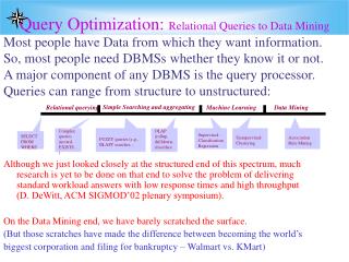
Relational Query Optimization
Relational Query Optimization. Implementation of single Relational Operations Choices depend on indexes, memory, stats,… Joins Blocked nested loops: simple, exploits extra memory Indexed nested loops: best if 1 rel small and one indexed Sort/Merge Join

Relational Query Optimization
E N D
Presentation Transcript
Relational Query Optimization • Implementation of single Relational Operations • Choices depend on indexes, memory, stats,… • Joins • Blocked nested loops: • simple, exploits extra memory • Indexed nested loops: • best if 1 rel small and one indexed • Sort/Merge Join • good with small amount of memory, bad with duplicates • Hash Join • fast (enough memory), bad with skewed data
sname rating > 5 bid=100 sid=sid Sailors Reserves Query Optimization Overview • Query can be converted to relational algebra • Rel. Algebra converted to tree, joins as branches • Each operator has implementation choices • Operators can also be applied in different order! SELECT S.sname FROM Reserves R, Sailors S WHERE R.sid=S.sid AND R.bid=100 AND S.rating>5 (sname)(bid=100 rating > 5) (Reserves Sailors)
Query Optimization Overview (cont) • Plan:Tree of R.A. ops (and some others) with choice of algorithm for each op. • Each operator typically implemented using a `pull’ interface: when an operator is `pulled’ for the next output tuples, it `pulls’ on its inputs and computes them. • Two main issues: • For a given query, what plans are considered? • Algorithm to search plan space for cheapest (estimated) plan. • How is the cost of a plan estimated? • Ideally: Want to find best plan. • Reality: Avoid worst plans!
Recall: Iterator Interface • A note on implementation: sname Relational operators at nodes support uniform iterator interface: Open( ), get_next( ), close( ) rating > 5 bid=100 sid=sid Sailors Reserves
Catalog Manager Cost-based Query Sub-System Select * From Blah B Where B.blah = blah Queries Usually there is a heuristics-based rewriting step before the cost-based steps. Query Parser Query Optimizer Plan Generator Plan Cost Estimator Schema Statistics Query Executor
Schema for Examples Sailors (sid: integer, sname: string, rating: integer, age: real) Reserves (sid: integer, bid: integer, day: dates, rname: string) • As seen in previous two lectures… • Reserves: • Each tuple is 40 bytes long, 100 tuples per page, 1000 pages. • Assume there are 100 boats • Sailors: • Each tuple is 50 bytes long, 80 tuples per page, 500 pages. • Assume there are 10 different ratings • Assume we have 5 pages in our buffer pool!
(On-the-fly) sname (On-the-fly) rating > 5 bid=100 (Page-Oriented Nested loops) sid=sid Reserves Sailors Motivating Example SELECT S.sname FROM Reserves R, Sailors S WHERE R.sid=S.sid AND R.bid=100 AND S.rating>5 • Cost: 500+500*1000 I/Os • By no means the worst plan! • Misses several opportunities: selections could have been `pushed’ earlier, no use is made of any available indexes, etc. • Goal of optimization: To find more efficient plans that compute the same answer. Plan:
(On-the-fly) sname (On-the-fly) bid=100 (On-the-fly) sname (Page-Oriented Nested loops) sid=sid (On-the-fly) rating > 5 bid=100 rating > 5 (On-the-fly) Reserves (Page-Oriented Nested loops) Sailors sid=sid Reserves Sailors Alternative Plans – Push Selects (No Indexes) 500,500 IOs 250,500 IOs
(On-the-fly) sname (On-the-fly) bid=100 (On-the-fly) sname (Page-Oriented Nested loops) sid=sid (Page-Oriented Nested loops) sid=sid rating > 5 (On-the-fly) Reserves bid = 100 rating > 5 Sailors (On-the-fly) (On-the-fly) Sailors Reserves Alternative Plans – Push Selects (No Indexes) 250,500 IOs 250,500 IOs
(On-the-fly) (On-the-fly) sname sname (On-the-fly) bid=100 rating > 5 (On-the-fly) (Page-Oriented Nested loops) (Page-Oriented Nested loops) sid=sid sid=sid rating > 5 (On-the-fly) Reserves bid=100 Sailors (On-the-fly) Sailors Reserves Alternative Plans – Push Selects (No Indexes) 6000 IOs 250,500 IOs
(On-the-fly) sname (On-the-fly) sname rating > 5 (On-the-fly) (Page-Oriented Nested loops) (Page-Oriented Nested loops) sid=sid sid=sid (Scan & Write to temp T2) rating > 5 bid=100 bid=100 Sailors (On-the-fly) (On-the-fly) Reserves Sailors Reserves Alternative Plans – Push Selects (No Indexes) 4250 IOs 1000 + 500+ 250 + (10 * 250) 6000 IOs
(On-the-fly) (On-the-fly) sname sname (Page-Oriented Nested loops) (Page-Oriented Nested loops) sid=sid sid=sid (Scan & Write to temp T2) (Scan & Write to temp T2) rating > 5 bid=100 bid=100 rating>5 (On-the-fly) (On-the-fly) Reserves Sailors Reserves Sailors Alternative Plans – Push Selects (No Indexes) 4250 IOs 4010 IOs 500 + 1000 +10 +(250 *10)
(On-the-fly) sname (Sort-Merge Join) sid=sid (Scan; (Scan; writeto write to rating > 5 bid=100 temp T2) tempT1) Reserves Sailors More Alternative Plans (No Indexes) • Main difference: Sort Merge Join • With 5 buffers, cost of plan: • Scan Reserves (1000) + write temp T1 (10 pages, if we have 100 boats, uniform distribution). • Scan Sailors (500) + write temp T2 (250 pages, if have 10 ratings). • Sort T1 (2*2*10), sort T2 (2*3*250), merge (10+250) • Total: 3560 page I/Os. • If use BNL join, join = 10+4*250, total cost = 2770. • Can also `push’ projections, but must be careful! • T1 has only sid, T2 only sid, sname: • T1 fits in 3 pgs, cost of BNL under 250 pgs, total < 2000.
(On-the-fly) sname More Alt Plans: Indexes (On-the-fly) rating > 5 (Index Nested Loops, with pipelining ) sid=sid • With clustered index on bid of Reserves, we get 100,000/100 = 1000 tuples on 1000/100 = 10 pages. • INL with outer not materialized. (Use hash Index, do not write to temp) bid=100 Sailors • Projecting out unnecessary fields from outer doesn’t help. Reserves • Join column sid is a key for Sailors. • At most one matching tuple, unclustered index on sid OK. • Decision not to push rating>5 before the join is based on • availability of sid index on Sailors. • Cost: Selection of Reserves tuples (10 I/Os); then, for each, • must get matching Sailors tuple (1000*1.2); total 1210 I/Os.
What is needed for optimization? • A closed set of operators • Relational ops (table in, table out) • Encapsulation based on iterators • Plan space, based on • Based on relational equivalences • Cost Estimation, based on • Cost formulas • Size estimation, based on • Catalog information on base tables • Selectivity (Reduction Factor) estimation • A search algorithm • To sift through the plan space based on cost!
Summary • Query optimization is an important task in a relational DBMS. • Must understand optimization in order to understand the performance impact of a given database design (relations, indexes) on a workload (set of queries). • Two parts to optimizing a query: • Consider a set of alternative plans. • Must prune search space; typically, left-deep plans only. • Must estimate cost of each plan that is considered. • Must estimate size of result and cost for each plan node. • Key issues: Statistics, indexes, operator implementations.
Query Optimization • Query can be dramatically improved by changing access methods, order of operators. • Iterator interface • Cost estimation • Size estimation and reduction factors • Statistics and Catalogs • Relational Algebra Equivalences • Choosing alternate plans • Multiple relation queries • Will focus on “System R”-style optimizers
Highlights of System R Optimizer • Impact: • Most widely used currently; works well for < 10 joins. • Cost estimation: • Very inexact, but works ok in practice. • Statistics, maintained in system catalogs, used to estimate cost of operations and result sizes. • Considers combination of CPU and I/O costs. • More sophisticated techniques known now. • Plan Space: Too large, must be pruned. • Only the space of left-deep plans is considered. • Cartesian products avoided.
D C B A Query Blocks: Units of Optimization SELECT S.sname FROM Sailors S WHERE S.age IN (SELECT MAX (S2.age) FROM Sailors S2 GROUP BY S2.rating) • An SQL query is parsed into a collection of queryblocks, and these are optimized one block at a time. • Nested blocks are usually treated as calls to a subroutine, made once per outer tuple. (This is an over-simplification, but serves for now.) Outer block Nested block • For each block, the plans considered are: • All available access methods, for each reln in FROM clause. • All left-deep join trees(i.e., right branchalways a base table, considerall join orders and join methods.)
Schema for Examples Sailors (sid: integer, sname: string, rating: integer, age: real) Reserves (sid: integer, bid: integer, day: dates, rname: string) • Reserves: • Each tuple is 40 bytes long, 100 tuples per page, 1000 pages. 100 distinct bids. • Sailors: • Each tuple is 50 bytes long, 80 tuples per page, 500 pages. 10 ratings, 40,000 sids.
Translating SQL to Relational Algebra SELECT S.sid, MIN (R.day) FROM Sailors S, Reserves R, Boats B WHERE S.sid = R.sid AND R.bid = B.bid AND B.color = “red” AND S.rating = ( SELECT MAX (S2.rating) FROM Sailors S2) GROUP BY S.sid HAVING COUNT (*) >= 2 For each sailor with the highest rating (over all sailors), and at least two reservations for red boats, find the sailor id and the earliest date on which the sailor has a reservation for a red boat.
p S.sid, MIN(R.day) (HAVING COUNT(*)>2 ( GROUP BY S.Sid ( B.color = “red” S.rating = val( Sailors Reserves Boats)))) s Ù Translating SQL to Relational Algebra SELECT S.sid, MIN (R.day) FROM Sailors S, Reserves R, Boats B WHERE S.sid = R.sid AND R.bid = B.bid AND B.color = “red” AND S.rating = ( SELECT MAX (S2.rating) FROM Sailors S2) GROUP BY S.sid HAVING COUNT (*) >= 2 Inner Block
Relational Algebra Equivalences • Allow us to choose different join orders and to `push’ selections and projections ahead of joins. • Selections: • This means we can do joins in any order. ( ) (Cascade) ( ) ( ) s º s s R . . . R Ù Ù c 1 . . . cn c 1 cn (Commute) • Projections: (Cascade) (Associative) R (S T) (R S) T • Joins: (Commute) (R S) (S R)
More Equivalences • A projection commutes with a selection that only uses attributes retained by the projection. • Selection between attributes of the two arguments of a cross-product converts cross-product to a join. • A selection on just attributes of R commutes with R S. (i.e., (R S) (R) S ) • Similarly, if a projection follows a join R S, we can `push’ it by retaining only attributes of R (and S) that are needed for the join or are kept by the projection.
Cost Estimation • For each plan considered, must estimate cost: • Must estimate costof each operation in plan tree. • Depends on input cardinalities. • We’ve already discussed how to estimate the cost of operations (sequential scan, index scan, joins, etc.) • Must estimate size of result for each operation in tree! • Use information about the input relations. • For selections and joins, assume independence of predicates. • In System R, cost is boiled down to a single number consisting of #I/O + factor * #CPU instructions • Q: Is “cost” the same as estimated “run time”?
Statistics and Catalogs • Need information about the relations and indexes involved. Catalogstypically contain at least: • # tuples (NTuples) and # pages (NPages) per rel’n. • # distinct key values (NKeys) for each index. • low/high key values (Low/High) for each index. • Index height (IHeight) for each tree index. • # index pages (INPages) for each index. • Catalogs updated periodically. • Updating whenever data changes is too expensive; lots of approximation anyway, so slight inconsistency ok. • More detailed information (e.g., histograms of the values in some field) are sometimes stored.
Size Estimation and Reduction Factors SELECT attribute list FROM relation list WHERE term1 AND ... ANDtermk • Consider a query block: • Maximum # tuples in result is the product of the cardinalities of relations in the FROM clause. • Reduction factor (RF) associated with eachtermreflects the impact of the term in reducing result size. Resultcardinality = Max # tuples * product of all RF’s. • RF usually called “selectivity”
Result Size Estimation • Resultcardinality = Max # tuples * product of all RF’s. (Implicit assumption that values are uniformly distributed and terms are independent!) • Term col=value (given index I on col ) RF = 1/NKeys(I) • Term col1=col2 (This is handy for joins too…) RF = 1/MAX(NKeys(I1), NKeys(I2)) • Term col>value RF = (High(I)-value)/(High(I)-Low(I)) • Note, if missing indexes, assume 1/10!!!
- age attribute values between 0 and 14- total count of all frequencies = 45- consider: age > 13
Equiwidth and equidepth histograms • in equiwidth histograms the range is divided in subranges of equal size • in equidepth histograms the ranges are choosen such that the number of tuples within in subrange (bucket) is equal • we assume that the distribution within a histogram bucket is uniform.
IBM DB2, Informix, Microsoft SQL Server, Oracle 8, and Sybase ASE all use histograms to estimate query characteristics such as result size and cost. As an example, Sybase ASE uses one-dimensional, equidepth histograms with some special attention paid to high frequency values so that their count is estimated accurately.
Think through estimation for joins • Does the above make sense for joins? • Q: Given a join of R and S, what is the range of possible result sizes (in #of tuples)? • If join is on a key for R (and a Foreign Key in S)? • A common case, can treat it specially • General case: join on {A} ({A} is key for neither) • estimate each tuple r of R generates NTuples(S)/NKeys(A,S) result tuples, so… NTuples(R) * NTuples(S)/NKeys(A,S) • but can also consider it starting with S, yielding: NTuples(S) * NTuples(R)/NKeys(A,R) • If these two estimates differ, take the lower one! • Q: Why?
Enumeration of Alternative Plans • There are two main cases: • Single-relation plans • Multiple-relation plans • For queries over a single relation, queries consist of a combination of selects, projects, and aggregate ops: • Each available access path (file scan / index) is considered, and the one with the least estimated cost is chosen. • The different operations are essentially carried out together (e.g., if an index is used for a selection, projection is done for each retrieved tuple, and the resulting tuples are pipelined into the aggregate computation).
Cost Estimates for Single-Relation Plans • Index I on primary key matches selection: • Cost is Height(I)+1 for a B+ tree. • Clustered index I matching one or more selects: • (NPages(I)+NPages(R)) * product of RF’s of matching selects. • Non-clustered index I matching one or more selects: • (NPages(I)+NTuples(R)) * product of RF’s of matching selects. • Sequential scan of file: • NPages(R). • Recall:Must also charge for duplicate elimination if required
Example SELECT S.sid FROM Sailors S WHERE S.rating=8 • If we have an index on rating: • Cardinality = (1/NKeys(I)) * NTuples(R) = (1/10) * 40000 tuples • Clustered index: (1/NKeys(I)) * (NPages(I)+NPages(R)) = (1/10) * (50+500) = 55 pages are retrieved. (This is the cost.) • Unclustered index: (1/NKeys(I)) * (NPages(I)+NTuples(R)) = (1/10) * (50+40000) = 401 pages are retrieved. • If we have an index on sid: • Would have to retrieve all tuples/pages. With a clustered index, the cost is 50+500, with unclustered index, 50+40000. • Doing a file scan: • We retrieve all file pages (500).
Evaluating Selections without Disjunction • intersecting rid sets • Oracle 8 uses several techniques to do rid set intersection for selections with AND. One is to AND bitmaps. • hash join of indexes • Example: sal < 5 ^ price > 30 • indexes on sal and price, we can join the indexes on the rid column, considering only entries that satisfy the given selection conditions. • Microsoft SQL Server implements rid set intersection through index joins.
D D C C D B A C B A B A Queries Over Multiple Relations • Fundamental decision in System R: only left-deep join treesare considered. • As the number of joins increases, the number of alternative plans grows rapidly; we need to restrict the search space. • Left-deep trees allow us to generate all fully pipelined plans. • Intermediate results not written to temporary files. • Not all left-deep trees are fully pipelined (e.g., SM join).
Enumeration of Left-Deep Plans • Left-deep plans differ only in the order of relations, the access method for each relation, and the join method for each join. • Enumerated using N passes (if N relations joined): • Pass 1: Find best 1-relation plan for each relation. • Pass 2: Find best way to join result of each 1-relation plan (as outer) to another relation. (All 2-relation plans.) • Pass N: Find best way to join result of a (N-1)-relation plan (as outer) to the N’th relation. (All N-relation plans.) • For each subset of relations, retain only: • Cheapest plan overall, plus • Cheapest plan for each interesting order of the tuples.
A Note on “Interesting Orders” • An intermediate result has an “interesting order” if it is sorted by any of: • ORDER BY attributes • GROUP BY attributes • Join attributes of yet-to-be-planned joins
Enumeration of Plans (Contd.) • An N-1 way plan is not combined with an additional relation unless there is a join condition between them, unless all predicates in WHERE have been used up. • i.e., avoid Cartesian products if possible. • ORDER BY, GROUP BY, aggregates etc. handled as a final step, using either an `interestingly ordered’ plan or an additonal sort/hash operator. • In spite of pruning plan space, this approach is still exponential in the # of tables. • Recall that in practice, COST considered is #IOs + factor * CPU Inst
Sid, COUNT(*) AS numbes GROUPBYsid sid=sid Sailors bid=bid Reserves Color=red Boats Sailors: Hash, B+ on sid Reserves: Clustered B+ tree on bid B+ on sid Boats B+, Hash on color Example Select S.sid, COUNT(*) AS number FROM Sailors S, Reserves R, Boats B WHERE S.sid = R.sid AND R.bid = B.bid AND B.color = “red” GROUP BY S.sid • Pass1: Best plan(s) for accessing each relation • Reserves, Sailors: File Scan • Q: What about Clustered B+ on Reserves.bid??? • Boats: B+ tree & Hash on color
Pass 1 • Best plan for accessing each relation regarded as the first relation in an execution plan • Reserves, Sailors: File Scan • Boats: B+ tree & Hash on color
Pass 2 • For each of the plans in pass 1, generate plans joining another relation as the inner, using all join methods (and matching inner access methods) • File Scan Reserves (outer) with Boats (inner) • File Scan Reserves (outer) with Sailors (inner) • File Scan Sailors (outer) with Boats (inner) • File Scan Sailors (outer) with Reserves (inner) • Boats hash on color with Sailors (inner) • Boats Btree on color with Sailors (inner) • Boats hash on color with Reserves (inner) (sort-merge) • Boats Btree on color with Reserves (inner) (BNL) • Retain cheapest plan for each pair of relations
Pass 3 and beyond • For each of the plans retained from Pass 2, taken as the outer, generate plans for the next join • eg Boats hash on color with Reserves (bid) (inner) (sortmerge)) inner Sailors (B-tree sid) sort-merge • Then, add the cost for doing the group by and aggregate: • This is the cost to sort the result by sid, unless it has already been sorted by a previous operator. • Then, choose the cheapest plan
Nested Queries • The unit of optimization in a typical system is a query block, and nested queries are dealt with using some form of nested loops evaluation. SELECT S.sname FROM Sailors S WHERE S.rating = ( SELECT MAX (S2.rating) FROM Sailors S2 ) • the nested subquery can be evaluated just once, yielding a single value. • if the highest rated sailor has a rating of 8, the WHERE clause is effectively modified to WHERE S.rating = 8
Nested Queries • the subquery may return a table SELECT S.sname FROM Sailors S WHERE S.sid IN ( SELECT R.sid FROM Reserves R WHERE R.bid = 103 ) • the nested subquery will be evaluated once, yielding a collection of sids • for each tuple of Sailors, we must check if the sid value is in the computed collection of sids; • this check entails a join of Sailors and the computed collection of sids;
SELECT S.sname FROM Sailors S WHERE EXISTS (SELECT * FROM Reserves R WHERE R.bid=103 AND R.sid=S.sid) Nested Queries • Nested block is optimized independently, with the outer tuple considered as providing a selection condition. • Outer block is optimized with the cost of `calling’ nested block computation taken into account. • Implicit ordering of these blocks means that some good strategies are not considered. The non-nested version of the query is typically optimized better. Nested block to optimize: SELECT * FROM Reserves R WHERE R.bid=103 AND R.sid= outer value Equivalent non-nested query: SELECT S.sname FROM Sailors S, Reserves R WHERE S.sid=R.sid AND R.bid=103
Nested Queries • the approach to nested subqueries is not set-oriented. A join is seen as a scan of the outer relation with a selection on the inner subquery for each outer tuple. • if there is an index on the sid field of Reserves, a good strategy might be to do an index nested loops join with Sailors as the outer relation and Reserves as the inner relation, and to apply the selection on bid on-the-fly. However, this option is not considered when optimizing the version of the query that uses IN because the nested subquery is fully evaluated as a first step; that is, Reserves tuples that meet the bid selection are retrieved first.
Nested Queries • A nested query often has an equivalent query without nesting, and a correlated query often has an equivalent query without correlation. • A typical SQL optimizer is likely to find a much better evaluation strategy if it is given the unnested or `decorrelated' version of the example query than it would if it were given either of the nested versions of the query. • Many current optimizers cannot recognize the equivalence of these queries and transform one of the nested versions to the nonnested form.