Download
1 / 17
170 likes | 257 Vues
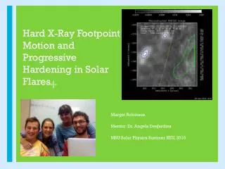
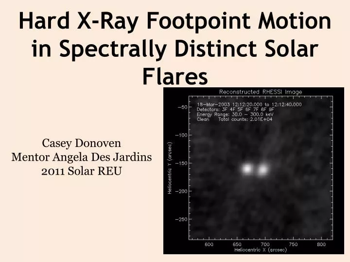
Hard X-Ray Footpoint Motion in Spectrally Distinct Solar Flares . Casey Donoven Mentor Angela Des Jardins 2011 Solar REU. Overview. Image the footpoints of solar flares using the RHESSI satellite Use the images to calculate the speed of the footpoints

E N D
Hard X-Ray Footpoint Motion in Spectrally Distinct Solar Flares Casey Donoven Mentor Angela Des Jardins 2011 Solar REU
Overview • Image the footpoints of solar flares using the RHESSI satellite • Use the images to calculate the speed of the footpoints • Look for correlation between footpoint speed and the spectrum of the non-thermal X-rays from the flare
Background • Solar flares form when loops of magnetic field lines undergo magnetic reconnection. • Charged particles precipitate out toward the ends of the loop, along the magnetic field lines. • Upon collision with the chromosphere, these particles undergo non-thermal, bremsstrahlung radiation and emit • X-rays. • The ratio of high energy to low energy non-thermal radiation will climb and fall throughout the flare, also known as spectral hardening and softening.
Background Solar energetic particles (SEPs) are thought to originate by being accelerated along open field lines in front of coronal mass ejections (CMEs). SEPs can range from tens of keV to GeV, meaning these particle have enough energy to be harmful to astronauts and satellites in orbit.
Background • ReuvanRamaty High Energy Solar Spectroscopic Imager (RHESSI)- • 3 keV to 17 MeV • Spatial resolution of up to 2 arcseconds • Images using 9 rotating modulation collimators and Fourier transforms
Motivation In a 2009 paper by James A. Grayson, SämKrucker, and R. P. Lin, a statistical correlation was found between the hardening of solar flares and SEP events. SHS- Soft hard soft SHH- Soft hard harder*
Mission -Investigate footpoint motion in relation to spectral hardening and SEP events Due to the coupling of the footpoints of flares and magnetic reconnection, a link between their motion and SEP events would challenge current theory and support the idea that SEPs originate near the flare or are simply causally related to the flare itself, not the CME.
Methods Using the RHESSI Gui, I analyzed the lightcurves of larger flares. I would then begin to make images over times with enough counts. Problems: Low counts, attenuator changes, looptop sources, lost data, possible multiple flares, only one footpoint, slow
Methods I contoured the images using a level which only the footpoints would be captured. The gui would write the data from the contour, such as time, centroid, peak flux, etc..., into a text file where I would clean it.
Methods I contoured the images using a level which only the footpoints would be captured. The gui would write the data from the contour, such as time, centroid, peak flux, etc..., into a text file where I would clean it.
Calculations • In order to maintain accuracy in calculating the speed of the footpoints, I wrote a program that filled several roles for me: • Returned all values in a structure • Included a conversion from arcseconds to kilometers • Calculated the standard deviation of all relevant data sets • The speeds were unreasonable so we decided that smoothing the data was the best option.
Calculations Method 1: Averaging I first tried averaging consecutive positions and times. My program allowed for the number of coordinates per block to be an input. I plotted speed vs. block size to determine when the speed was most accurate.
Calculations Method 2: Fitting Polynomials In this method, I fit polynomials to the data and used the derivative to calculate the speed. We used the chi squared fitness statistic and visual aids to determine the right degree of polynomial. Plots are of May 29, 2003 flare.
Results * There were two flares on this day. This is the 10:24 flare.
Conclusion Fitting polynomials to the data produced what we believe to be the best results for smoothing the centroid motion. However, due to a lack of data, a statistical analysis cannot be done. Further work would simply include analyzing more flares and create a consistent method of selecting the degree of polynomial to be used. In cases where the RHESSI data is insufficient, the TRACE satellite could be used to observe the motion of the ribbon instead.