Download
1 / 79
800 likes | 1.18k Vues
Overview of Assembly Language. Chapter 9 S. Dandamudi. Assembly language statements Data allocation Where are the operands? Addressing modes Register Immediate Direct Indirect Data transfer instructions mov , xchg , and xlat PTR directive. Overview of assembly language instructions

E N D
Overview of Assembly Language Chapter 9 S. Dandamudi
Assembly language statements Data allocation Where are the operands? Addressing modes Register Immediate Direct Indirect Data transfer instructions mov, xchg, and xlat PTR directive Overview of assembly language instructions Arithmetic Conditional Logical Shift Rotate Defining constants EQU and = directives Macros Illustrative examples Outline S. Dandamudi
Assembly Language Statements • Three different classes • Instructions • Tell CPU what to do • Executable instructions with an op-code • Directives (or pseudo-ops) • Provide information to assembler on various aspects of the assembly process • Non-executable • Do not generate machine language instructions • Macros • A shorthand notation for a group of statements • A sophisticated text substitution mechanism with parameters S. Dandamudi
Assembly Language Statements (cont’d) • Assembly language statement format: [label] mnemonic [operands] [;comment] • Typically one statement per line • Fields in [ ] are optional • label serves two distinct purposes: • To label an instruction • Can transfer program execution to the labeled instruction • To label an identifier or constant • mnemonicidentifies the operation (e.g., add, or) • operands specify the data required by the operation • Executable instructions can have zero to three operands S. Dandamudi
Assembly Language Statements (cont’d) • comments • Begin with a semicolon (;) and extend to the end of the line Examples repeat: inc result; increment result CR EQU 0DH; carriage return character • White space can be used to improve readability repeat: inc result S. Dandamudi
Data Allocation • Variable declaration in a high-level language such as C char response int value float total double average_value specifies • Amount storage required (1 byte, 2 bytes, …) • Label to identify the storage allocated (response, value, …) • Interpretation of the bits stored (signed, floating point, …) • Bit pattern 1000 1101 1011 1001 is interpreted as • -29,255 as a signed number • 36,281 as an unsigned number S. Dandamudi
Data Allocation (cont’d) • In assembly language, we use the define directive • Define directive can be used • To reserve storage space • To label the storage space • To initialize • But no interpretation is attached to the bits stored • Interpretation is up to the program code • Define directive goes into the .DATA part of the assembly language program • Define directive format [var-name] D? init-value [,init-value],... S. Dandamudi
Data Allocation (cont’d) • Five define directives DB Define Byte ;allocates 1 byte DW Define Word ;allocates 2 bytes DD Define Doubleword ;allocates 4 bytes DQ Define Quadword ;allocates 8 bytes DT Define Ten bytes ;allocates 10 bytes Examples sorted DB ’y’ response DB ? ;no initialization value DW 25159 float1 DD 1.234 float2 DQ 123.456 S. Dandamudi
Data Allocation (cont’d) • Multiple definitions can be abbreviated Example message DB ’B’ DB ’y’ DB ’e’ DB 0DH DB 0AH can be written as message DB ’B’,’y’,’e’,0DH,0AH • More compactly as message DB ’Bye’,0DH,0AH S. Dandamudi
Data Allocation (cont’d) • Multiple definitions can be cumbersome to initialize data structures such as arrays Example To declare and initialize an integer array of 8 elements marks DW 0,0,0,0,0,0,0,0 • What if we want to declare and initialize to zero an array of 200 elements? • There is a better way of doing this than repeating zero 200 times in the above statement • Assembler provides a directive to do this (DUP directive) S. Dandamudi
Data Allocation (cont’d) • Multiple initializations • The DUP assembler directive allows multiple initializations to the same value • Previous marks array can be compactly declared as marks DW 8 DUP (0) Examples table1 DW 10 DUP (?) ;10 words, uninitialized message DB 3 DUP (’Bye!’) ;12 bytes, initialized ; as Bye!Bye!Bye! Name1 DB 30 DUP (’?’) ;30 bytes, each ; initialized to ? S. Dandamudi
Data Allocation (cont’d) • The DUP directive may also be nested Example stars DB 4 DUP(3 DUP (’*’),2 DUP (’?’),5 DUP (’!’)) Reserves 40-bytes space and initializes it as ***??!!!!!***??!!!!!***??!!!!!***??!!!!! Example matrix DW 10 DUP (5 DUP (0)) defines a 10X5 matrix and initializes its elements to 0 This declaration can also be done by matrix DW 50 DUP (0) S. Dandamudi
Data Allocation (cont’d) Symbol Table • Assembler builds a symbol table so we can refer to the allocated storage space by the associated label Example .DATAnameoffset value DW 0value 0 sum DD 0sum 2 marks DW 10 DUP (?)marks 6 message DB ‘The grade is:’,0message 26 char1 DB ?char1 40 S. Dandamudi
Data Allocation (cont’d) Correspondence to C Data Types Directive C data type DB char DW int, unsigned DD float, long DQ double DT internal intermediate float value S. Dandamudi
Data Allocation (cont’d) LABEL Directive • LABEL directive provides another way to name a memory location • Format: name LABEL type typecan be BYTE 1 byte WORD 2 bytes DWORD 4 bytes QWORD 8 bytes TWORD 10 bytes S. Dandamudi
Data Allocation (cont’d) LABEL Directive Example .DATA count LABEL WORD Lo-count DB 0 Hi_count DB 0 .CODE... mov Lo_count,AL mov Hi_count,CL • count refers to the 16-bit value • Lo_count refers to the low byte • Hi_count refers to the high byte S. Dandamudi
Where Are the Operands? • Operands required by an operation can be specified in a variety of ways • A few basic ways are: • operand in a register • register addressing mode • operand in the instruction itself • immediate addressing mode • operand in memory • variety of addressing modes • direct and indirect addressing modes • operand at an I/O port • discussed in Chapter 19 S. Dandamudi
Where Are the Operands? (cont’d) Register addressing mode • Operand is in an internal register Examples mov EAX,EBX ; 32-bit copy mov BX,CX ; 16-bit copy mov AL,CL ; 8-bit copy • The mov instruction mov destination,source copies data from source to destination S. Dandamudi
Where Are the Operands? (cont’d) Register addressing mode (cont’d) • Most efficient way of specifying an operand • No memory access is required • Instructions using this mode tend to be shorter • Fewer bits are needed to specify the register • Compilers use this mode to optimize code total := 0 for (i = 1 to 400) total = total + marks[i] end for • Mapping total and i to registers during the for loop optimizes the code S. Dandamudi
Where Are the Operands? (cont’d) Immediate addressing mode • Data is part of the instruction • Ooperand is located in the code segment along with the instruction • Efficient as no separate operand fetch is needed • Typically used to specify a constant Example mov AL,75 • This instruction uses register addressing mode for destination and immediate addressing mode for the source S. Dandamudi
Where Are the Operands? (cont’d) Direct addressing mode • Data is in the data segment • Need a logical address to access data • Two components: segment:offset • Various addressing modes to specify the offset component • offset part is called effective address • The offset is specified directly as part of instruction • We write assembly language programs using memory labels (e.g., declared using DB, DW, LABEL,...) • Assembler computes the offset value for the label • Uses symbol table to compute the offset of a label S. Dandamudi
Where Are the Operands? (cont’d) Direct addressing mode (cont’d) Examples mov AL,response • Assembler replaces response by its effective address (i.e., its offset value from the symbol table) mov table1,56 • table1 is declared as table1 DW 20 DUP (0) • Since the assembler replaces table1 by its effective address, this instruction refers to the first element of table1 • In C, it is equivalent to table1[0] = 56 S. Dandamudi
Where Are the Operands? (cont’d) Direct addressing mode (cont’d) • Problem with direct addressing • Useful only to specify simple variables • Causes serious problems in addressing data types such as arrays • As an example, consider adding elements of an array • Direct addressing does not facilitate using a loop structure to iterate through the array • We have to write an instruction to add each element of the array • Indirect addressing mode remedies this problem S. Dandamudi
Where Are the Operands? (cont’d) Indirect addressing mode • The offset is specified indirectly via a register • Sometimes called register indirect addressing mode • For 16-bit addressing, the offset value can be in one of the three registers: BX, SI, or DI • For 32-bit addressing, all 32-bit registers can be used Example mov AX,[BX] • Square brackets [ ] are used to indicate that BX is holding an offset value • BX contains a pointer to the operand, not the operand itself S. Dandamudi
Where Are the Operands? (cont’d) • Using indirect addressing mode, we can process arrays using loops Example: Summing array elements • Load the starting address (i.e., offset) of the array into BX • Loop for each element in the array • Get the value using the offset in BX • Use indirect addressing • Add the value to the running total • Update the offset in BX to point to the next element of the array S. Dandamudi
Where Are the Operands? (cont’d) Loading offset value into a register • Suppose we want to load BX with the offset value of table1 • We cannot write mov BX,table1 • Two ways of loading offset value • Using OFFSET assembler directive • Executed only at the assembly time • Using lea instruction • This is a processor instruction • Executed at run time S. Dandamudi
Where Are the Operands? (cont’d) Loading offset value into a register (cont’d) • Using OFFSET assembler directive • The previous example can be written as mov BX,OFFSET table1 • Using lea (load effective address) instruction • The format of lea instruction is lea register,source • The previous example can be written as lea BX,table1 S. Dandamudi
Where Are the Operands? (cont’d) Loading offset value into a register (cont’d) Which one to use -- OFFSET or lea? • Use OFFSET if possible • OFFSET incurs only one-time overhead (at assembly time) • lea incurs run time overhead (every time you run the program) • May have to use lea in some instances • When the needed data is available at run time only • An index passed as a parameter to a procedure • We can write lea BX,table1[SI] to load BX with the address of an element of table1 whose index is in SI register • We cannot use the OFFSET directive in this case S. Dandamudi
Default Segments • In register indirect addressing mode • 16-bit addresses • Effective addresses in BX, SI, or DI is taken as the offset into the data segment (relative to DS) • For BP and SP registers, the offset is taken to refer to the stack segment (relative to SS) • 32-bit addresses • Effective address in EAX, EBX, ECX, EDX, ESI, and EDI is relative to DS • Effective address in EBP and ESP is relative to SS • push and pop are always relative to SS S. Dandamudi
Default Segments (cont’d) • Default segment override • Possible to override the defaults by using override prefixes • CS, DS, SS, ES, FS, GS • Example 1 • We can use add AX,SS:[BX] to refer to a data item on the stack • Example 2 • We can use add AX,DS:[BP] to refer to a data item in the data segment S. Dandamudi
Data Transfer Instructions • We will look at three instructions • mov(move) • Actually copy • xchg (exchange) • Exchanges two operands • xlat (translate) • Translates byte values using a translation table • Other data transfer instructions such as movsx (move sign extended) movzx (move zero extended) are discussed in Chapter 12 S. Dandamudi
Data Transfer Instructions (cont’d) The mov instruction • The format is mov destination,source • Copies the value from source to destination • source is not altered as a result of copying • Both operands should be of same size • source and destination cannot both be in memory • Most Pentium instructions do not allow both operands to be located in memory • Pentium provides special instructions to facilitate memory-to-memory block copying of data S. Dandamudi
Data Transfer Instructions (cont’d) The mov instruction • Five types of operand combinations are allowed: Instruction type Example mov register,register mov DX,CX mov register,immediate mov BL,100 mov register,memory mov BX,count mov memory,register mov count,SI mov memory,immediate mov count,23 • The operand combinations are valid for all instructions that require two operands S. Dandamudi
Data Transfer Instructions (cont’d) Ambiguous moves: PTR directive • For the following data definitions .DATA table1 DW 20 DUP (0) status DB 7 DUP (1) the last two mov instructions are ambiguous mov BX,OFFSET table1 mov SI,OFFSET status mov [BX],100 mov [SI],100 • Not clear whether the assembler should use byte or word equivalent of 100 S. Dandamudi
Data Transfer Instructions (cont’d) Ambiguous moves: PTR directive • The PTR assembler directive can be used to clarify • The last two mov instructions can be written as mov WORD PTR [BX],100 mov BYTE PTR [SI],100 • WORD and BYTE are called type specifiers • We can also use the following type specifiers: DWORD for doubleword values QWORD for quadword values TWORD for ten byte values S. Dandamudi
Data Transfer Instructions (cont’d) The xchg instruction • The syntax is xchg operand1,operand2 Exchanges the values of operand1 and operand2 Examples xchg EAX,EDX xchg response,CL xchg total,DX • Without the xchg instruction, we need a temporary register to exchange values using only the mov instruction S. Dandamudi
Data Transfer Instructions (cont’d) The xchg instruction • The xchginstruction is useful for conversion of 16-bit data between little endian and big endian forms • Example: mov AL,AH converts the data in AX into the other endian form • Pentium provides bswap instruction to do similar conversion on 32-bit data bswap 32-bit register • bswap works only on data located in a 32-bit register S. Dandamudi
Data Transfer Instructions (cont’d) The xlat instruction • The xlatinstruction translates bytes • The format is xlatb • To use xlat instruction • BX should be loaded with the starting address of the translation table • AL must contain an index in to the table • Index value starts at zero • The instruction reads the byte at this index in the translation table and stores this value in AL • The index value in AL is lost • Translation table can have at most 256 entries (due to AL) S. Dandamudi
Data Transfer Instructions (cont’d) The xlat instruction Example: Encrypting digits Input digits: 0 1 2 3 4 5 6 7 8 9 Encrypted digits: 4 6 9 5 0 3 1 8 7 2 .DATA xlat_table DB ’4695031872’ ... .CODE mov BX,OFFSET xlat_table GetCh AL sub AL,’0’ ;converts input character to index xlatb ;AL = encrypted digit character PutCh AL ... S. Dandamudi
Pentium Assembly Instructions • Pentium provides several types of instructions • Brief overview of some basic instructions: • Arithmetic instructions • Jump instructions • Loop instruction • Logical instructions • Shift instructions • Rotate instructions • These instructions allow you to write reasonable assembly language programs S. Dandamudi
Arithmetic Instructions INC and DEC instructions • Format: inc destination dec destination • Semantics: destination = destination +/- 1 • destination can be 8-, 16-, or 32-bit operand, in memory or register • No immediate operand • Examples inc BX dec value S. Dandamudi
Arithmetic Instructions (cont’d) Add instructions • Format: add destination,source • Semantics: destination = destination + source • Examples add EBX,EAX add value,35 • inc EAX is better than add EAX,1 • inc takes less space • Both execute at about the same speed S. Dandamudi
Arithmetic Instructions (cont’d) Add instructions • Addition with carry • Format: adc destination,source • Semantics: destination = destination + source + CF • Example: 64-bit addition add EAX,ECX ; add lower 32 bits adc EBX,EDX ; add upper 32 bits with carry • 64-bit result in EBX:EAX S. Dandamudi
Arithmetic Instructions (cont’d) Subtract instructions • Format: sub destination,source • Semantics: destination = destination - source • Examples sub EBX,EAX sub value,35 • dec EAX is better than sub EAX,1 • dec takes less space • Both execute at about the same speed S. Dandamudi
Arithmetic Instructions (cont’d) Subtract instructions • Subtract with borrow • Format: sbb destination,source • Semantics: destination = destination - source - CF • Like the adc, sbb is useful indealing with more than 32-bit numbers • Negation neg destination • Semantics: destination = 0 - destination S. Dandamudi
Arithmetic Instructions (cont’d) CMP instruction • Format: cmp destination,source • Semantics: destination - source • destination and source are not altered • Useful to test relationship (>, =) between two operands • Used in conjunction with conditional jump instructions for decision making purposes • Examples cmp EBX,EAX cmp count,100 S. Dandamudi
Unconditional Jump • Format: jmp label • Semantics: • Execution is transferred to the instruction identified by label • Target can be specified in one of two ways • Directly • In the instruction itself • Indirectly • Through a register or memory • Discussed in Chapter 12 S. Dandamudi
Example Two jump instructions Forward jump jmp CX_init_done Backward jump jmp repeat1 Programmer specifies target by a label Assembler computes the offset using the symbol table . . . mov CX,10 jmp CX_init_done init_CX_20: mov CX,20 CX_init_done: mov AX,CX repeat1: dec CX . . . jmp repeat1 . . . Unconditional Jump (cont’d) S. Dandamudi
Unconditional Jump (cont’d) • Address specified in the jump instruction is not the absolute address • Uses relative address • Specifies relative byte displacement between the target instruction and the instruction following the jump instruction • Displacement is w.r.t the instruction following jmp • Reason: IP points to this instruction after reading jump • Execution of jmp involves adding the displacement value to current IP • Displacement is a signed 16-bit number • Negative value for backward jumps • Positive value for forward jumps S. Dandamudi
Target Location • Inter-segment jump • Target is in another segment CS = target-segment (2 bytes) IP = target-offset (2 bytes) • Called far jumps (needs five bytes to encode jmp) • Intra-segment jumps • Target is in the same segment IP = IP + relative-displacement (1 or 2 bytes) • Uses 1-byte displacement if target is within -128 to +127 • Called short jumps (needs two bytes to encode jmp) • If target is outside this range, uses 2-byte displacement • Called near jumps (needs three bytes to encode jmp) S. Dandamudi