Price Competition
360 likes | 381 Vues
Price Competition. Introduction. In a wide variety of markets firms compete in prices Internet access Restaurants Consultants Financial services With monopoly setting price or quantity first makes no difference In oligopoly it matters a great deal

Price Competition
E N D
Presentation Transcript
Price Competition Chapter 10: Price Competition
Introduction • In a wide variety of markets firms compete in prices • Internet access • Restaurants • Consultants • Financial services • With monopoly setting price or quantity first makes no difference • In oligopoly it matters a great deal • nature of price competition is much more aggressive the quantity competition Chapter 10: Price Competition
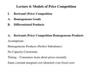
Price Competition: Bertrand • In the Cournot model price is set by some market clearing mechanism • An alternative approach is to assume that firms compete in prices: this is the approach taken by Bertrand • Leads to dramatically different results • Take a simple example • two firms producing an identical product (spring water?) • firms choose the prices at which they sell their products • each firm has constant marginal cost of c • inverse demand is P = A – B.Q • direct demand is Q = a – b.P with a = A/B and b= 1/B Chapter 10: Price Competition
Bertrand competition • We need the derived demand for each firm • demand conditional upon the price charged by the other firm • Take firm 2. Assume that firm 1 has set a price of p1 • if firm 2 sets a price greater than p1 she will sell nothing • if firm 2 sets a price less than p1 she gets the whole market • if firm 2 sets a price of exactly p1 consumers are indifferent between the two firms: the market is shared, presumably 50:50 • So we have the derived demand for firm 2 • q2 = 0 if p2 > p1 • q2 = (a – bp2)/2 if p2 = p1 • q2 = a – bp2 if p2 < p1 Chapter 10: Price Competition
Bertrand competition 2 p2 • This can be illustrated as follows: There is a jump at p2 = p1 • Demand is discontinuous • The discontinuity in demand carries over to profit p1 a - bp1 a q2 (a - bp1)/2 Chapter 10: Price Competition
Bertrand competition 3 Firm 2’s profit is: p2(p1,, p2) = 0 if p2 > p1 p2(p1,, p2) = (p2 - c)(a - bp2) if p2 < p1 For whatever reason! p2(p1,, p2) = (p2 - c)(a - bp2)/2 if p2 = p1 Clearly this depends on p1. Suppose first that firm 1 sets a “very high” price: greater than the monopoly price of pM = (a +c)/2b Chapter 10: Price Competition
What price should firm 2 set? Bertrand competition 4 Firm 2 will only earn a positive profit by cutting its price to (a + c)/2b or less With p1 > (a + c)/2b, Firm 2’s profit looks like this: The monopoly price At p2 = p1 firm 2 gets half of the monopoly profit Firm 2’s Profit So firm 2 should just undercut p1 a bit and get almost all the monopoly profit p2 < p1 What if firm 1 prices at (a + c)/2b? p2 = p1 p2 > p1 p1 c (a+c)/2b Firm 2’s Price Chapter 10: Price Competition
Bertrand competition 5 Now suppose that firm 1 sets a price less than (a + c)/2b Firm 2’s profit looks like this: What price should firm 2 set now? As long as p1 > c, Firm 2 should aim just to undercut firm 1 Firm 2’s Profit Of course, firm 1 will then undercut firm 2 and so on Then firm 2 should also price at c. Cutting price below costgains the whole market but loses money on every customer p2 < p1 What if firm 1 prices at c? p2 = p1 p2 > p1 p1 (a+c)/2b c Firm 2’s Price Chapter 10: Price Competition
Bertrand competition 6 • We now have Firm 2’s best response to any price set by firm 1: • p*2 = (a + c)/2b if p1 > (a + c)/2b • p*2 = p1 - “something small” if c < p1< (a + c)/2b • p*2 = c if p1< c • We have a symmetric best response for firm 1 • p*1 = (a + c)/2b if p2 > (a + c)/2b • p*1 = p2 - “something small” if c < p2< (a + c)/2b • p*1 = c if p2< c Chapter 10: Price Competition
Bertrand competition 7 The best response function for firm 1 The best response function for firm 2 These best response functions look like this p2 R1 The Bertrand equilibrium has both firms charging marginal cost R2 (a + c)/2b The equilibrium is with both firms pricing at c c p1 c (a + c)/2b Chapter 10: Price Competition
Bertrand Equilibrium: modifications • The Bertrand model makes clear that competition in prices is very different from competition in quantities • Since many firms seem to set prices (and not quantities) this is a challenge to the Cournot approach • But the extreme version of the difference seems somewhat forced • Two extensions can be considered • impact of capacity constraints • product differentiation Chapter 10: Price Competition
Capacity Constraints • For the p = c equilibrium to arise, both firms need enough capacity to fill all demand at p = c • But when p = c they each get only half the market • So, at the p = c equilibrium, there is huge excess capacity • So capacity constraints may affect the equilibrium • Consider an example • daily demand for skiing on Mount Norman Q = 6,000 – 60P • Q is number of lift tickets and P is price of a lift ticket • two resorts: Pepall with daily capacity 1,000 and Richards with daily capacity 1,400, both fixed • marginal cost of lift services for both is $10 Chapter 10: Price Competition
The Example • Is a price P = c = $10 an equilibrium? • total demand is then 5,400, well in excess of capacity • Suppose both resorts set P = $10: both then have demand of 2,700 • Consider Pepall: • raising price loses some demand • but where can they go? Richards is already above capacity • so some skiers will not switch from Pepall at the higher price • but then Pepall is pricing above MC and making profit on the skiers who remain • so P = $10 cannot be an equilibrium Chapter 10: Price Competition
The example 2 • Assume that at any price where demand at a resort is greater than capacity there is efficient rationing • serves skiers with the highest willingness to pay • Then can derive residual demand • Assume P = $60 • total demand = 2,400 = total capacity • so Pepall gets 1,000 skiers • residual demand to Richards with efficient rationing is Q = 5000 – 60P or P = 83.33 – Q/60 in inverse form • marginal revenue is then MR = 83.33 – Q/30 Chapter 10: Price Competition
The example 3 • Residual demand and MR: Price • Suppose that Richards sets P = $60. Does it want to change? $83.33 Demand $60 • since MR > MC Richards does not want to raise price and lose skiers MR $36.66 • since QR = 1,400 Richards is at capacity and does not want to reduce price $10 MC 1,400 Quantity • Same logic applies to Pepall so P = $60 is a Nash equilibrium for this game. Chapter 10: Price Competition
Capacity constraints again • Logic is quite general • firms are unlikely to choose sufficient capacity to serve the whole market when price equals marginal cost • since they get only a fraction in equilibrium • so capacity of each firm is less than needed to serve the whole market • but then there is no incentive to cut price to marginal cost • So the efficiency property of Bertrand equilibrium breaks down when firms are capacity constrained Chapter 10: Price Competition
Product differentiation • Original analysis also assumes that firms offer homogeneous products • Creates incentives for firms to differentiate their products • to generate consumer loyalty • do not lose all demand when they price above their rivals • keep the “most loyal” Chapter 10: Price Competition
An example of product differentiation Coke and Pepsi are similar but not identical. As a result, the lower priced product does not win the entire market. Econometric estimation gives: QC = 63.42 - 3.98PC + 2.25PP MCC = $4.96 QP = 49.52 - 5.48PP + 1.40PC MCP = $3.96 There are at least two methods for solving for PC and PP Chapter 10: Price Competition
Bertrand and product differentiation Method 1: Calculus Profit of Coke: pC = (PC - 4.96)(63.42 - 3.98PC + 2.25PP) Profit of Pepsi: pP = (PP - 3.96)(49.52 - 5.48PP + 1.40PC) Differentiate with respect to PC and PP respectively Method 2: MR = MC Reorganize the demand functions PC = (15.93 + 0.57PP) - 0.25QC PP = (9.04 + 0.26PC) - 0.18QP Calculate marginal revenue, equate to marginal cost, solve for QC and QP and substitute in the demand functions Chapter 10: Price Competition
Bertrand and product differentiation 2 Both methods give the best response functions: PC = 10.44 + 0.2826PP PP The Bertrand equilibrium is at their intersection Note that these are upward sloping RC PP = 6.49 + 0.1277PC These can be solved for the equilibrium prices as indicated RP $8.11 B $6.49 The equilibrium prices are each greater than marginal cost PC $10.44 $12.72 Chapter 10: Price Competition
Bertrand competition and the spatial model • An alternative approach: spatial model of Hotelling • a Main Street over which consumers are distributed • supplied by two shops located at opposite ends of the street • but now the shops are competitors • each consumer buys exactly one unit of the good provided that its full price is less than V • a consumer buys from the shop offering the lower full price • consumers incur transport costs of t per unit distance in travelling to a shop • Recall the broader interpretation • What prices will the two shops charge? Chapter 10: Price Competition
Bertrand and the spatial model xm marks the location of the marginal buyer—one who is indifferent between buying either firm’s good What if shop 1 raises its price? Assume that shop 1 sets price p1 and shop 2 sets price p2 Price Price p’1 p2 p1 x’m xm All consumers to the left of xm buy from shop 1 And all consumers to the right buy from shop 2 xm moves to the left: some consumers switch to shop 2 Shop 1 Shop 2 Chapter 10: Price Competition
Price Price p2 p1 xm Shop 1 Shop 2 Bertrand and the spatial model 2 p1 + txm = p2 + t(1 - xm) 2txm = p2 - p1 + t How is xm determined? xm(p1, p2) = (p2 - p1 + t)/2t This is the fraction of consumers who buy from firm 1 There are N consumers in total So demand to firm 1 is D1 = N(p2 - p1 + t)/2t Chapter 10: Price Competition
Bertrand equilibrium Profit to firm 1 is p1 = (p1 - c)D1 = N(p1 - c)(p2 - p1 + t)/2t This is the best response function for firm 1 p1 = N(p2p1 - p12 + tp1 + cp1 - cp2 -ct)/2t Solve this for p1 Differentiate with respect to p1 N p1/ p1 = (p2 - 2p1 + t + c) = 0 2t p*1 = (p2 + t + c)/2 This is the best response function for firm 2 What about firm 2? By symmetry, it has a similar best response function. p*2 = (p1 + t + c)/2 Chapter 10: Price Competition
Bertrand equilibrium 2 p2 p*1 = (p2 + t + c)/2 R1 p*2 = (p1 + t + c)/2 2p*2 = p1 + t + c R2 = p2/2 + 3(t + c)/2 c + t p*2 = t + c (c + t)/2 p*1 = t + c Profit per unit to each firm is t p1 (c + t)/2 c + t Aggregate profit to each firm is Nt/2 Chapter 10: Price Competition
Bertrand competition 3 • Two final points on this analysis • t is a measure of transport costs • it is also a measure of the value consumers place on getting their most preferred variety • when t is large competition is softened • and profit is increased • when t is small competition is tougher • and profit is decreased • Locations have been taken as fixed • suppose product design can be set by the firms • balance “business stealing” temptation to be close • against “competition softening” desire to be separate Chapter 10: Price Competition
Strategic complements and substitutes q2 • Best response functions are very different with Cournot and Bertrand Firm 1 Cournot • they have opposite slopes • reflects very different forms of competition • firms react differently e.g. to an increase in costs Firm 2 q1 p2 Firm 1 Firm 2 Bertrand p1 Chapter 10: Price Competition
q2 Firm 1 Cournot Firm 2 q1 p2 Firm 1 Firm2 Bertrand p1 Strategic complements and substitutes • suppose firm 2’s costs increase • this causes Firm 2’s Cournot best response function to fall • at any output for firm 1 firm 2 now wants to produce less • firm 1’s output increases and firm 2’s falls aggressive response by firm1 passive response by firm1 • Firm 2’s Bertrand best response function rises • at any price for firm 1 firm 2 now wants to raise its price • firm 1’s price increases as does firm 2’s Chapter 10: Price Competition
Strategic complements and substitutes 2 • When best response functions are upward sloping (e.g. Bertrand) we have strategic complements • passive action induces passive response • When best response functions are downward sloping (e.g. Cournot) we have strategic substitutes • passive actions induces aggressive response • Difficult to determine strategic choice variable: price or quantity • output in advance of sale – probably quantity • production schedules easily changed and intense competition for customers – probably price Chapter 10: Price Competition
Empirical Application: Brand Competition and Consumer Preferences • As noted earlier, products can be differentiated horizontally or vertically • In many respects, which type of differentiation prevails reflects underlying consumer preferences • Are the meaningful differences between consumers about what makes for quality and not about what quality is worth (Horizontal Differentiation); Or • Are the meaningful differences between consumers not about what constitutes good quality but about how much extra quality should be valued (Vertical Differentiation) Chapter 10: Price Competition
Brand Competition & Consumer Preferences 2 • Consider the study of the retail gasoline market in southern California by Hastings (2004) • Gasoline is heavily branded. Established brands like Chevron and Exxon-Mobil have contain special, trademarked additives that are not found in discount brands, e.g. RaceTrak. • In June 1997, the established brand Arco gained control of 260 stations in Southern California formerly operated by the discount independent, Thrifty • By September of 1997, the acquired stations were converted to Arco stations. What effect did this have on branded gasoline prices? Chapter 10: Price Competition
Brand Competition & Consumer Preferences 3 • If consumers regard Thrifty as substantially different in quality from the additive brands, then losing the Thrifty stations would not hurt competition much while the entry of 260 established Arco stations would mean a real increase in competition for branded gasoline and those prices should fall. • If consumers do not see any real quality differences worth paying for but simply valued the Thrifty stations for providing a low-cost alternative, then establish brand prices should rise after the acquisition. • So, behavior of gasoline prices before and after the acquisition tells us something about preferences. Chapter 10: Price Competition
Brand Competition & Consumer Preferences 4 • Tracking differences in price behavior over time is tricky though • Hastings (2004) proceeds by looking at gas stations that competed with Thrifty’s before the acquisition (were within 1 mile of a Thrifty) and ones that do not. She asks if there is any difference in the response of the prices at these two types of stations to the conversion of the Thrifty stations • Presumably, prices for both types were different after the acquisition than they were before it. The question is, is there a difference between the two groups in these before-and-after differences? For this reason, this approach is called a difference-in-differences model. Chapter 10: Price Competition
Brand Competition & Consumer Preferences 5 Hastings observes prices for each station in Feb, June, Sept. and December of 1997, i.e., before and after the conversion. She runs a regression explaining station i’s price in each of the four time periods, t pit = Constant + i+ 1Xit + 2Zit+ 3Ti+ eit i is an intercept term different for each that controls for differences between each station unrelated to time Xit is 1 if station i competes with a Thrifty at time t and 0 otherwise. Zit is 1 if station i competes with a station directly owned by a major brand but 0 if it is a franchise. Ti is a sequence of time dummies equal reflecting each of the four periods. This variable controls for the pure effect of time on the prices at all stations. Chapter 10: Price Competition
Brand Competition & Consumer Preferences 6 The issue is the value of the estimated coefficient 1 Ignore the contractual variable Zit for the moment and consider two stations: firm 1that competed with a Thrifty before the conversion and firm 2 that did not. In the pre-conversion periods, Xitis positive for firm 1 but zero for firm 2. Over time, each firm will change its price because of common factors that affect them over time. However, firm 1 will also change is price because for the final two observations, Xit is zero. Before After Difference Firm 1: αi +β1αi + time effects - β1 + time effects Firm 2: αjαj + time effects time effects Chapter 10: Price Competition
Brand Competition & Consumer Preferences 6 Thus, the estimated coefficient 1 captures the difference in movement over time between firm 1 and firm 2. Hastings (2004) estimates 1 to be about -0.05. That is, firms that competed with a Thrifty saw their prices rise by about 5 cents more over time than did other firms Before the conversion, prices at stations that competed against Thrifty’s were about 2 to 3 cents below those that did not. After the removal of the Thrifty’s, however, they had prices about 2 to 3 cents higher than those that did not. Conversion of the Thrifty’s to Arco stations did not intensify competition among the big brands. Instead, it removed a lost cost alternative. Chapter 10: Price Competition