Network Inference
Network Inference. Umer Zeeshan Ijaz. 1. Overview. Introduction Application Areas cDNA Microarray EEG/ECoG Network Inference Pair-wise Similarity Measures Cross-correlation STATIC


Network Inference
E N D
Presentation Transcript
Network Inference Umer Zeeshan Ijaz 1
Overview • Introduction • Application Areas • cDNA Microarray • EEG/ECoG • Network Inference • Pair-wise Similarity Measures • Cross-correlation STATIC • Coherence STATIC • Autoregressive • Granger Causality STATIC • Probabilistic Graphical Models • Directed • Kalman-filtering based EM algorithm STATIC • Undirected • Kernel-weighted logistic regression method DYNAMIC • Graphical Lasso-model STATIC
Cross-correlation based(1) For a pair of time series xi[t] and xj[t] of lengths n, the sample correlation at lag τ Measure of Coupling is the maximum cross correlation: Use P-Value test to compare zij with a standard normal distribution with mean zero and variance 1
Cross-correlation based (2) Significance test: ANALYTIC METHOD Use Fisher Transformation: the resulting distribution is normal and has the standard deviation of Use scaled value that is expected to behave like the maximum of the absolute value of a sequence of random numbers. Using now established results for statistics of this form, we obtain therefore that *M. A. Kramer, U. T. Eden, S. S. Cash, E. D. Kolaczyk, Network inference with confidence from multivariate time series. Physical review E 79, 061916, 2009
Cross-correlation based (3) Significance test: FREQUENCY DOMAIN BOOTSTRAP METHOD • Compute the power spectrum (Hanning tapered) of each series and average these power spectra from all the time series • Compute the standardized and whitened residuals for each time series • For each bootstrap replicate, RESAMPLE WITH REPLACEMENT and compute the surrogate data • Compute such instances and calculate maximum cross-correlation for each pair of nodes i and j • Finally compare the bootstrap distribution and assign a p-value
Cross-correlation based (4) False Detection Rate Test • Order m=N(N-1)/2 p-values • Choose FDR level q • Compare each to critical value and find the maximum i such that • We reject the null hypothesis that time series and are uncoupled for *M. A. Kramer, U. T. Eden, S. S. Cash, and E. D. Kolaczyk. Network inference with confidence from multivariate time series, Physics Review E 79(061916), 1-13, 2009
Coherence based Coherence: Signals are fully correlated with constant phase shifts, although they may show difference in amplitude Cross-phase spectrum: Provides information on time-relationships between two signals as a function of frequency. Phase displacement may be converted into time displacement
Coherence based(2) *S. Weiss, and H. M. Mueller. The contribution of EEG coherence to the investigation of language, Brain and Language 85(2), 325-343, 2003
Granger Causality Directed Transfer Function: Directional influences between any given pair of channels in a multivariate data set Bivariate autoregressive process If the variance of the prediction error is reduced by the inclusion of other series, then based on granger causality, one depends on another. Now taking the fourier transform Granger causality from channel j to i:
Kalman Filter - State Space Model (State Variable Model; State Evolution Model) State Equation Measurement Equation Measurement Update(Filtering) Time Update(Prediction)
Probabilistic graphical models(1) Joint distribution over a set Bayesian Networks associate with each variable a conditional probability The resulting product is of the form A B P(C|A,B) A B 0 1 0 0 0.9 0.1 0 1 0.2 0.8 1 0 0.9 0.1 1 1 0.01 0.99 D C E
EM Algorithm: Predicting gene regulatory network Constructing the network:
EM Algorithm: Predicting gene regulatory network(2) Conditional distribution of state and observables Factorization rule for bayesian network Unknowns in the system
EM Algorithm: Predicting gene regulatory network(4) Construct the likelihood Construct the likelihood Marginalize with respect to x and introducing a distribution Q
Kalman filter based: Inferring network from microarray expression data(5) Let’s say we want to compute C
Kalman filter based: Inferring network from microarray expression data(9) Experimental Results: A standard T-Cell activation model *Claudia Rangel, John Angus, Zoubin Ghahramani, Maria Lioumi, Elizabeth Sotheran, Alessia Gaiba, David L. Wild, Francesco Falciani: Modeling T-cell activation using gene expression profiling and state-space models. Bioinformatics 20(9): 1361-1372 (2004)
Probabilistic graphical models(2) Markov Networks represent joint distribution as a product of potentials D A A B π1(A,B) 0 0 1.0 0 1 0.5 1 0 0.5 1 1 2.0 C B E
Kernel-weighted logistic regression method(1) Pair-wise Markov Random Field x6 x7 θθ56 θθ57 x1 x5 x8 θθ25 θθ48 Logistic Function θθ12 θθ54 x2 x4 θθ23 θθ34 x3 Log Likelihood Optimization problem
Kernel-weighted logistic regression method(3) Interaction between gene ontological groups related to developmental process undergoing dynamic rewiring. The weight of an edge between two ontological groups is the total number of connection between genes in the two groups. In the visualization, the width of an edge is propotional to the edge weight. The edge weight is thresholded at 30 so that only those interactions exceeding this number are displayed. The average network on left is produced by averaging the right side. In this case, the threshold is set to 20 *L. Song, M. Kolar, and E. P. Xing. KELLER: estimating time-varying interactions between genes. Bioinformatics 25, i128-i136, 2009
Graphical Lasso Model(1) *O. Banerjee, L. E. Ghaoui, A. d’Aspremont. Model selection through sparse maximum likelihood estimation for multivariate gaussian or binary data. Journal of Machine Language Research 101, 2007
Graphical Lasso Model(2) Solve the lasso problem for w12 over jth column one at a time *O. Banerjee, L. E. Ghaoui, A. d’Aspremont. Model selection through sparse maximum likelihood estimation for multivariate gaussian or binary data. Journal of Machine Language Research 101, 2007
Graphical Lasso Model(3) *Software under development @ Oxford Complex Systems Group with Nick Jones *Results shown for Google Trend Dataset
THE END 27