Dynamic Network Inference
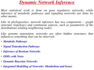
Dynamic Network Inference. Most statistical work is done on gene regulatory networks, while inference of metabolic pathways and signaling networks are done by other means.

Dynamic Network Inference
E N D
Presentation Transcript
Dynamic Network Inference Most statistical work is done on gene regulatory networks, while inference of metabolic pathways and signaling networks are done by other means. Like in phylogenetics, network inference has two components – graph structure (topology) and continuous aspects, such as parameters of the distributions relating neighboring nodes. Like genome annotation, networks are often hidden structures that influences something that can be observed. • Metabolic Pathways • Signal Transduction Pathways • Inference of Boolean Networks • ODEs with Noise • Dynamic Bayesian Networks • Integrated Modelling of Networks: Metabolism and Genes
Inferring Metabolic Pathways • Given reaction • Create atom to atom mapping between molecules Solvable by Subgraph Isomorphism Algorithms • Partial Injections • Partial Injections can be concatenated Arita (2000) Metabolic reconstruction using shortest path Simulation Practice and Theory8.1-2.109-12 Arita (2000) Graph Modelling of Metabolism JS Art Intel. 15.4.?? Boyer (2003) Ab Initia reconstruction of metabolic pathways Bioinformatics 19.2.26-34
Example:Tryptophan from 4-erythrose via Chorismate • Automaton generating paths with at least 6 carbons transferred and maximum length 6. • Bold paths corresponds to biological pathway.
Inferring Signalling Pathways Graph G=(E,V) with some some nodes real, some pseudo. Pseudo are non-observed, but simplifies explanation. Edges are labelled 0-excitation, 1 inhibition. A 0 C 1 1 B 0 Paths from i to j has parity weight of path modulo 2 Ecritical - set of experimentally verified interactions Albert et al. (2007) A Novel Method for Signal Trnasduction Network Inference from Indirect Experimental Evidence JCompuBiol. 14.7.927- Li et l. (2006) Predicting Essential Components of Signal Transduction Networks: A Dynamic Model of Guard Cell Abscisic Acid Signaling. PLOS Biol. 4.10.1732- Observations: Inhibition/Excitation relationships between all real pairs BTR – Binary Transitive Reduction: Find a subgraph E’ : Ecritical < E’ < E such that parity remains the same. PVC – Pseudo Vertex Collapse. Procedure to remove pseudovertices without changing parity. Questions: there might be several paths from i to j. The effect of i on j, depends on the state of other nodes – ie cannot be viewed in isolation
Abscisic Acid (ABA) Signaling and Simulations • Manually Curated • Inferred by Algorithm 54 vertices, 92 edges --- Identical strong connected component ---- 54 + 3 vertices, 84 edges Simulation: How large is proposed networks relative to theoretical lower bounds.
Reverse Engeneering Algorithm-Reveal Discrete known Generations No Noise Shannon Entropies: X Mutual Information: M(X,Y) = H(Y) – H(Y given X) = H(X)-H(X given Y) 3 2 Y For j=1 to k Find k-sets with significant mutual information. Assign rule. 1 4 H(X) = .97 D’haeseler et al.(2000) Genetic network Inference: from co-expression clustering to reverse engineering. Bioinformatics 16.8.707- H(Y) = 1.00 X 0 1 1 1 1 1 1 1 0 0 0 H(X,Y) = 1.85 Y 0 0 0 1 1 0 0 0 1 1 1 • 50 genes • Random firing rules • Thus network inference is easy. • However, it is not
BOOL-1, BOOL2, QNET1 Akutsu et al. (2000) Inferring qualitative relations in genetic networks and metabolic pathways. Bioinformatics 16.2.727- Bool-1 Algorithm For each gene do (n) For each boolean rule (<= k inputs) not violated, keep it. If O(22k[2k + a]log(n)) INPUT patterns are given uniformly randomly, BOOL-1 correctly identifies the underlying network with probability 1-n-a, where a is any fixed real number > 1. pnoise is the probability that experiment reports wrong boolean rule uniformly. Bool-2 Qualitative Network QNET Qnet X1 X2 Inhibition vj--!vi Activation vjvi Algorithm if (DXi* Xj <0) delete “n1 activatesn2”from E if (DXi* Xj >0) delete “n1 inhibitsn2”from E
ODEs with Noise This can be modeled by Where Feed forward loop (FFL) Z X Y If noise is given a distribution the problem is well defined and statistical estimation can be done Data and estimation Goodness of Fit and Significance Objective is to estimate from noisy measurements of expression levels Cao and Zhao (2008) “Estimating Dynamic Models for gene regulation networks” Bioinformatics 24.14.1619-24
Inference in the Presence of Knowledge Dynamic mass action systems on 10 components were sampled with a bias towards sparseness Kinetic parameters were sampled Dynamic trajectories were generated Normal noise was added Equation system minimizing SSE was chosen Adding deterministic knowledge was added Marton Munz -http://www.stats.ox.ac.uk/__data/assets/pdf_file/0016/4255/Munz_homepage.pdf - http://www.stats.ox.ac.uk/research/genome/projects
Gaussian Processes Definition: A Stochastic Process X(t) is a GP if all finite sets of time points, t1,t2,..,tk, defines stochastic variable that follows a multivariate Normal distribution, N(m,S), where m is the k-dimensional mean and S is the k*k dimensional covariance matrix. Examples: Brownian Motion: All increments are N( ,Dt) distributed. Dt is the time period for the increment. No equilibrium distribution. Ornstein-Uhlenbeck Process – diffusion process with centralizing linear drift. N( , ) as equilibrium distribution. One TF (transcription factor – black ball) (f(t)) whose concentration fluctuates over times influence k genes (xj) (four in this illustration) through their TFBS (transcription factor binding site - blue). The strength of its influence is described through a gene specific sensitivity, Sj. Dj– decay of gene j, Bj– production of gene j in absence of TF
Gaussian Processes Gaussian Processes are characterized by their mean and variances thus calculating these for xj and f at pairs of time, t and t’, points is a key objective Observable level Hidden and Gaussian time t t’ Correlation between two time points of f Correlation between two time points of same x’es Rattray, Lawrence et al. Manchester Correlation between two time points of different x’es Correlation between two time points of x and f This defines a prior on the observables Then observe and a posterior distribution is defined
Gaussian Processes Relevant Generalizations: Non-linear response function Multiple transcription factors Network relationship between genes Observations in Multiple Species Comments: Inference of Hidden Processes has strong similarity to genome annotation
Graphical Models Edges/Hyperedges – directed or undirected – determines the combined distribution on all nodes. Labeled Nodes: each associated a stochastic variable that can be observed or not. 2 2 1 1 3 3 4 4 • Conditional Independence • Gaussian • Correlation Graphs • Causality Graphs
Dynamic Bayesian Networks • Make a time series of of it • Model the observable as function of present network Take a graphical model Perrin et al. (2003) “Gene networks inference using dynamic Bayesian networks” Bioinformatics 19.suppl.138-48. Example: DNA repair Inference about the level of hidden variables can be made
Network Integration Modified from Ruppin Genome-scale integrated model for E. coli (Covert 2004) 1010 genes (104 TFs, 906 genes) 817 proteins 1083 reactions Regulatory state (Boolean vector) Metabolic state A genome scale computational study of the interplay between transcriptional regulation and metabolism. (T. Shlomi, Y. Eisenberg, R. Sharan, E. Ruppin) Molecular Systems Biology (MSB), 3:101, doi:10.1038/msb4100141, 2007 Chen-Hsiang Yeang and Martin Vingron, "A joint model of regulatory and metabolic networks" (2006). BMC Bioinformatics. 7, pp. 332-33.
Feasibility of Network Inference: Very Hard Why it is hard: • Data very noisy • Number of network topologies very large What could help: • Other sources of knowledge – experiments • Evolution • Declaring biology unknowable would be very radical Why poor network inference might be acceptable: • A biological conclusion defines a large set of networks What statistics can do • Conceptual clarification of problem • Optimal analysis of data • Power studies (how much data do you need) Statistics can’t draw conclusion if the data is insufficient or too noisy (I hope not)
Summary • Network Inference – topology and continuous parameters • Metabolic Pathways • Signal Transduction Pathways • Inference of Boolean Networks • ODEs with Noise • Dynamic Bayesian Networks • Integrated Modeling of Networks: Metabolism and Genes • Interpretation: From Integrative Genomics to Systems Biology: • Often the topology is assumed identical