Download
1 / 39
390 likes | 530 Vues
SR Theory of Electrodynamics for Relative Moving Charges. By James Keele, M.S.E.E . October 27, 2012. Special Theory of Relativity (SRT). Basic Postulates Relativity Principle(RP): “all inertial frames are totally equivalent for the performance of all physical experiments”

E N D
SR Theory of Electrodynamics for Relative Moving Charges By James Keele, M.S.E.E. October 27,2012
Special Theory of Relativity (SRT) Basic Postulates • Relativity Principle(RP): “all inertial frames are totally equivalent for the performance of all physical experiments” • “light travels rectilinearly with constant speed c in vacuum in every inertial frame”
Logic applied to the 2nd Postulate: Constancy of the Speed of Light. If Physicists accept the law, , and believe that and are constant in all inertia frames then must be constant in all inertial frames. Otherwise, if and/or are/is not constant in all inertial frames, because is not constant, then Postulated 1 is invalid because the electrodynamics laws of nature contain these constants.
Other Basic Considerations • The charge of an electron or proton is mathematically considered herein to be a point charge and does not have a finite size. • An uniform electric field exists about a stationary electric point charge, pervading the space equally in all directions and falling off in intensity at 1/r2. • Velocities are relative between interacting particles.
Other Basic Considerations Cont’d 4. The electric field of a moving charge pervades all the space of its inertial frame, thus having instant reaction with a charge in contact with it. Acceleration of a charge creates a new velocity that changes the electric field that spreads out over the new inertial frame at the speed of light. 5. The charge value, q, is invariant from one inertial frame to another. 6. A positive sign on the overall magnetic force represents repulsion while a negative sign represents attraction. 7. A negative sign must be entered into the equations for negative charges such as electrons. A positive sign must be entered into the equations for positive charges such as protons. This makes the direction of the overall force appear correctly as in 6above.
SRT Formalism Employed • Lorentz Transformation • Three Vectors: a(a1, a2, a3) (lower case) 3. Four Vectors: V(V1.V2.V3,V4) (Upper case) Four vector force formula: • The four vector force is good for transforming force between inertial frames and creating force laws. 5.
Mathematical Setup for Analysis of Force Between Relative Moving Charge Particles
Lorentz Force Law—Starting Point for the Four-Force SRT Transformation Relativist’s Starting Point Lorentz Force Law (Wrong) (1) Keele’s Starting Point (Right) (2) f=3-force, q=charge, e=electric field, v=relative velocity, h=magnetic field, c=velocity of light
Why Relativist’s Starting Point is Wrong 1. When we are just trying to derive the force between a stationary charge and a moving charge the Lorentz Force Law that contains the magnetic field is the wrong starting point. If we include the term that has the magnetic field and assume it comes from the moving charge itself, then we would be doing a transform from two different inertial frames which is a “no-no” in SRT. If the term involving the magnetic field arises from a separate source other than the moving charge, then the transform would work for the transform of magnetic field. But we are not doing that, so we can expect the magnetic force to fall out of the transform of just the moving charge’s electric field. This was found to be the case. The is the most important point of this whole presentation that shows where errors are made. 2. The regular Lorentz Force Law could be applicable in Cathode Ray Tube or accelerators where the source of the magnetic field is separate from the “magnetic field” created by the moving charge. You don’t start out in two different inertial frames. 3. An experiment performed by Keele with his results shows that his is the correct starting point. 4. The magnetic field h in (1) is derived from the Biot-Savart Law which was derived before the Old Ampere’s Law from current flowing in a wire. The magnetic field from a moving isolated charge is different from the magnetic field of a current element as will be shown in a later slide.
Transformation Results Relativist’s Results (3) Keele’s Results (4)
Length Contraction of e-field of Moving Electron as seen by a Stationary Particle
Magnetic Force Between Relative Moving Isolated Charges Total electric field and magnetic forces between the relative slow moving charges (after mathematical manipulations of (4) using the Binomial Theorem and eliminating higher orders of ) : (5) Subtracting the stationary electric field force from (5) we have the magnetic force: (6)
Current Element Length contraction of the spacing between charges in the current element increases the charge line density of the current element as seen by a stationary observer (γσ). Moving Electrons --- showing length contraction of each charge’s field and the length contraction of the spacing between the charges in the current element Stationary Electrons Stationary Protons
The Magnetic Force Law Between a Stationary Charge and a Stationary Current Element Include one more relativistic effect to (4) for a current element (current flowing in a short piece of a conductor): This effect is length contraction of the spacing between the current carrying electrons in the current element as seen by the stationary charge. This has the effect of increasing the charge density of the current carrying electrons in the current element. The result is: (7) Where σis the line charge density. Notice there is a small magnetic force on a stationary charge with respect to the current element.
The Magnetic Force Law Between Stationary Current Elements (Found to Be the Old Ampere’s Law) Eq. (7) is applied three times to the cross combinations of charges in the two current elements and then the resulting forces are added. The charges in (7) are replaced by resulting in the Old Ampere’s Law: (8) A study of this law reveals that successive current elements with current in the same direction repel each other. This fact has been demonstrated by experiments of Peter Graneau. This is an effect the Biot-Savart Law does not allow. Eq. (8) obeys Newtons 3rd Law whereas most other similar laws do not. They generally have to be integrated around a closed loop to have any applicability.
Equivalent Mathematical Form of Old Ampere’s Law Eq. (9) below is mathematically equivalent to Eq. (8) in the previous slide: (9) where = unit vector in the direction of r12and r12 = magnitude of the vector r12 joining the two current elements. The constants are k = 1/40 (0 = permittivity of free space) and c = speed of light. The I1 and I2are current magnitudes and ds1 and ds2 are current element lengths. The angles are: 1 = angle between ds1and r12; 2 = angle between ds2 and r12; = angle between the plane of ds2 with r12 and the plane of ds1with r12.
Experiment With the Old Ampere’s Law A simple experiment was performed on various shapes of one-turn coils. The inductance L of these coils was computer calculated using Ampere’s Law. Then the Inductance was measured by determining resonance of the inductor with a calibrated capacitor. The measured value of L is then compared with the computed value.
Method employed to measure inductance (Lm) of a coil Calibrated Capacitor Formulas: , Resonance Sine Wave Generator One-turn coil Scope Frequency Meter
One-turn solenoid set up for calculating its inductance using the old Ampere’s Law
Math showing how inductance may be calculated using a computer
Experimental Results • Measured and Calculated Results (Wire dia. = 0.635) • Name ds(mm) Lm (microhenries) Lc (microhenries) Δ % • Triangle 2.4 1.914819 1.909496 -0.28 • Circle 2.7 2.399168 2.396962 -0.09 • Square 2.8 2.717203 2.717502 0.01 • 3-D Square 3.2 3.222207 3.223535 0.04 • 3-D Tetra 3.1 3.760989 3.765264 0.11 Since no self-inductance relationship of ds was employed in the calculation of Lc, it is deduced quite appropriately from the above table that for the measured and calculated values to agree so closely, the internal inductance of the current element ds must be zero. Varying the ds length on either side of the ones presented above will produce a calculated value of Lc that will be above or below the measured value of Lm.
Computer modeling of a current element to show zero energy stored in its inductance The self-inductance of the current element was not added in the computer model for calculating the inductance of single-turn inductors of the various shapes, so the self-inductance needed to be verified to be zero. End Views of current element Current Element A square cross-section is used in the model to approximate the round cross-section area of the wire current element to make the math easier. Areas are made equal. The current element is divided up into many rectangular parallelpipeds.
Current Element Length A computer model of the current element using the inductance (energy storage) formulation of Ampere’s Law was created. It determined the length of the current element so that there would be no energy storage in it. (The energy stored in each current element was not added in the computer calculations of the previous slide.) The following table shows the comparison between the required length of ds for a match between the calculated values of L with the measured values of L. • Circle coil. Wire dia. a parameter. • Wire dia. (mm) Lm (microhenries) ds (mm) required ds (mm) calculated • for Lc match for zero inductance in • current element model • 0.254 2.747 1 1.08 • 0.635 2.3992.8 2.71 • 2.134 1.944 12 9.1
Some Conclusions From Experiment 1. The old Ampere Law is the correct one. • The other magnetic laws derived above: force between relative moving charges, and the force between a charge and current element are correct since they preceded in derivation of the Old Ampere’s Law. • The SRT derivations of these laws are correct.
Some Applications • Arc Welding • Radio Wave Propagation • Study of Elementary Particles 4. Gravity
Arc Welding A study of the plasma current flow in the arc gap suggests the relative moving positive and negative ions will be pulled together greater than when stationary, and thus will emit energy. (This is analogous to an electron in a hydrogen atom falling from a higher orbit to a lower orbit.) It may be possible to “burn” the material of the plasma this way and thus emit more energy than is output from the welding machine.
Radio Wave Propagation Eq. (7) appropriately modified appears to be a natural for the expression of the magnetic field of a propagated radio wave. (7) Modified by: Remove q1 to go back to the magnetic e-field. Also the following: , , , (10) This magnetic field acts on a charge like an electric field. Further development is beyond the scope of my present intentions.
E-field of Dipole Antenna E-field is like the e-field between capacitor plates. Dipole Antenna e-field
Study of Elementary Particles Eq. (4) can be used in a Bohr Atom like model for elementary particles since the equations is good for up to the speed of light: (4)
Gravity If the gravity can be considered to be a field, and if the gravity field has similar characteristics to an electric field (but much smaller in amplitude), and if the heavenly bodies are treated as mathematical points, then the gravity field of a heavenly body will have the four-force Lorentz Transformation given by Eq. (11). (11)
Gravity Cont’d For slow relative moving heavenly bodies (earth in orbit about the sun for example) then Eq. (11) may be reduced to: (12) This is a new law of gravity.
Gravity Cont’d Eq. (12) was tested in a computer program to see if the excess force (in addition to the Newton gravity law) would produce the Mercury Perihelion Advance. (12)
Gravity Cont’d It did. Table below show the computed results: Expressed in arc seconds per 100 Earth years. (If Mercury’s advance was measured relative to Earth’s then Mercury’s Advance would be 42.3 calculated according to the computer model.)
Uses of New Gravity Law • May explain why rockets launched vertically travel further than predicted by Newton’s gravity law. • Use in accelerating universe ongoing studies. • Weight of a vertically rotating disc will be non-uniform: The top and bottom will be heavier, and the sides will be lighter. A horizontal spinning disc should weigh more than the same disc spinning vertically.
Summary of Derived Laws Magnetic Force Between: Relative Moving Isolated Charges: Stationary Charge and Current Element: Two Current Elements (Old Ampere’s Law): Total Gravity Force BetweenTwo Masses:
Reasons that these Laws are correct: • The old Ampere’s law was derived from SRT and found to be the correct one from the experiments performed. • The other two magnetic laws are fall-outs of the steps to derive the old Ampere’s, therefore they can be taken as correct. • The gravity law was derived by analogy with SRT applied to e-field of an isolated charge. The excess gravity force thus created was found by calculation to be responsible for the perihelion advances of the planets by computer computation. Therefore this law is correct.