Download
1 / 15
170 likes | 334 Vues
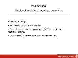
2nd meeting: Multilevel modeling: intra class correlation Subjects for today: Multilevel data base construction The difference between single level OLS regression and Multilevel analysis Multilevel analysis: the intra class correlation (ICC). What we have learned first meeting:

E N D
2nd meeting: • Multilevel modeling: intra class correlation • Subjects for today: • Multilevel data base construction • The difference between single level OLS regression and Multilevel analysis • Multilevel analysis: the intra class correlation (ICC)
What we have learned first meeting: • When we like to say something about higher level units like Indonesian districts or countries it is best to use multilevel analysis, because we use the right standard error and correct number of observations. • We need a data file with samples at district level and within district level we need samples from individuals: • Individual District body height • 1 Bandung 150 • 2 Bandung 145 • 3 Bandung 156 • 4 Majalengka 118 • 5 Majalengka 174 • 6 Majalengka 156 • 7 Serang 167 • 8 Serang 153 • 9 Serang 145 • 10 District X 144 • 11 District X 177 • 12 District X 188 2
Because we like to incorporate level 2 variables as well to explain why districts (or countries) differ. The data file look like this (welfare included): Individual District body height Welfare (in € per capita) 1 Bandung 150 300 2 Bandung 145 300 3 Bandung 156 300 4 Majalengka 118 100 5 Majalengka 174 100 6 Majalengka 156 100 7 Serang 167 200 8 Serang 153 200 9 Serang 145 200 10 District X 144 500 11 District X 177 500 12 District X 188 500 HOW TO GET THAT RIGHT? 3
First we have to get the welfare data for Indonesian districts: Can be found at Central Bureau for Statistics or other internet sites Second we like to have them in a SPSS readable data file (for instance an Excel file (Microsoft Office) or SPSS file like SAV or POR files). Third we must connect the welfare data to the individual data: In SPSS called a file Individual data: 1 Bandung 2 Bandung 3 Bandung 4 Serang 5 Serang Contextual data: Bandung 300 Serang 200 In SPSS called a table 4
SPSS Syntax to construct multilevel data files: GET FILE= "c:\multilevelmodeling\welfare.sav". * Watch it: data MUST be sorted by country first!!. sort cases by district. SAVE OUTFILE= "c:/multilevelmodeling/welfare.sav". GET FILE= "c:\multilevelmodeling\all_individuals.sav". * Watch it: sort data MUST be sorted by district first!!. sort cases by district. SAVE OUTFILE= "c:/multilevelmodeling/all_individuals.sav". match files table= "c:/ multilevelmodeling\welfare.sav" /file= "c:/multilevelmodeling/all_individuals.sav" /by district. EXE. 5
Ok, we have our data ready, what’s next? First we like to know whether there is variation WITHIN districts and variation BETWEEN districts: 6
In Mlwin we have something simular: first we have an equation with the within variance: Y = a + e ij where Y = dependent variable, a = intercept, e ij = within variance (error in regression analysis) i=individual, j=level2 (district) Second we have an equation with the between variance: a = B 0j + u j where B0j = intercept, u j = between variance Substituting a in the first equation gives: Y = B0 j + e ij + u 0j A multilevel null model !!! So in plain words: all individuals scores (Y ij) depend upon some figure (B O j + some individual variation + some level 2 variation. 7
Yij = B 0j + e 0ij + u 0j for two individuals in Bandung: Y Mean in Bandung Overall mean across the population of districts X 8
Now suppose that all districts have the same mean body weight: Then the between variance = 0. Suppose that all individuals within a district have all the same weight: Then the within variance = 0. In many research there is both within and between variance or both level 1 and level 2 variance. The total variance of course is level 1 variance + level 2 variance. Now suppose that all individuals are relatively closely clustered arond their district (or Group) means then the so-called intra class correlation is said to be high: ICC = level 2 variance / total variance (=variance level 1 and 2) ICC is always between 0 (only level 1 variance, no clustering) and 1 (only level 2 variance) 9
Now down to business. We have data (name SCHOOL23.sav, see our site, data used with kind permission from I. Kreft and J. De Leeuw. Introducing Multilevel Modeling. Sage Publications, 1998.) from 23 schools including 519 pupils and we have a math test als Y variabele. We like to know the between en within variances. * SPSS syntax: mixed math /random intercept | subject(school) covtype(un) /print solution g testcov /method ml. ICC= 24.85/ 24.85 + 81.23 = .23 10
We can also test with a Chi-square test whether ICC is significant. This way of testing is recommended, because it has NOT the normality assumption from a z-test. In Mlwin you can use Chi square testing because the difference between two -2 loglikelihoods is Chi-square distributed. Say we have a model with only level 1 variance with -2 loglikehood of 1600 and the same model but now both level 1 and 2 variance parameters: -2 loglikelihood will be equal or lower! So -2 loglikihood figures are a measures of fit: the lower it is the better the models fits the data. Because the difference in -2 loglikelihood between the models can be zero or higher, the test probability must be devided by 2! Note: On our site we included a brief instruction about statistical testing in MlwiN. 12
Model with one level only: Test whether ICC is significant or whether level 2 variance is significant different from zero we perform a Chi-square test: -2 loglikelihood from 1 level model - -2 loglikelihood from 2 level model: 3933.064 – 3800.776 = 132 with 1 df. Which is highly significant. This test is superior to the Z-test in SPSS because the latter uses an estimate for the standard error. Note: we test one sided because outcome is always zero or higher. 13
Let us assume that the difference between the -2 loglikihoods is 10. We have 1 df, because we added one extra parameter, which is the level 2 variance. The Chi-square distribution looks something like this: In fact we must divide 0.00156 by 2 to get the correct p=value, but the original p is already very low. The conclusion being that beyond reasonable doubt there is level 2 variance or ICC > 0! 14
Testing in MLwin with Chi-square (more info in document about testing, see: ‘statistical testing in Mlwin.pdf’. Note that 0.0015654 must be divided by 2 voor level 2 variance testing Type cprob 10 1 and press [Enter] 15