Download
1 / 45
450 likes | 692 Vues
Central dogma. Central dogma of biology DNA RNA pre-mRNA mRNA Protein. DNA:. CGAACAAACCTCGAACCTGCT. Translation. Basic molecular biology. Transcription. mRNA:. GCU UGU UUA CGA. Polypeptide:. Ala Cys Leu Arg. Transcription. End modification. Splicing.

E N D
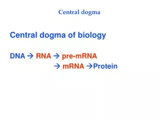
Central dogma Central dogma of biology DNA RNA pre-mRNA mRNA Protein
DNA: CGAACAAACCTCGAACCTGCT Translation Basic molecular biology Transcription mRNA: GCU UGU UUA CGA Polypeptide: Ala Cys Leu Arg
Transcription End modification Splicing Transport Translation Less basic molecular biology
RNA Biological Sample Test Sample Test Sample Reference PE Cy3 Cy5 ARRAY ARRAY Oligonucleotide Synthesis cDNA Clone (LIBRARY) PCR Product Microarray technology Ramaswamy and Golub, JCO
Microarray technology Oligonucleotide cDNA Lockhart and Winzler 2000
Microarray experiment Yeast experiment
Analytic challenge When the science is not well understood, resort to statistics: Infer cancer genetics by analyzing microarray data from tumors Ultimate goal: discover the genetic pathways of cancers Immediate goal: models that discriminate tumor types or treatment outcomes and determine genes used in model Basic difficulty: few examples 20-100, high-dimensionality 7,000-16,000 genes measured for each sample, ill-posed problem Curse of dimensionality: Far too few examples for so many dimensions to predict accurately
Cancer Diagnosis Acute Myeloblastic Leukemia v Acute Lymphoblastic Leukemia
Cancer Classification 38 examples of Myeloid and Lymphoblastic leukemias Affymetrix human 6800, (7128 genes including control genes) 34 examples to test classifier Results: 33/34 correct d perpendicular distance from hyperplane d Test data
Two gene example: two genes measuring Sonic Hedgehog and TrkC Coregulation and kernels Coregulation: the expression of two genes must be correlated for a protein to be made, so we need to look at pairwise correlations as well as individual expression Size of feature space: if there are 7,000 genes, feature space is about 24 million features, so the fact that feature space is never computed is important
Gene coregulation Nonlinear SVM helps when the most informative genes are removed, Informative as ranked using Signal to Noise (Golub et al). • Genes removed errors • 1st order 2nd order 3rd order polynomials • 0 1 1 1 • 10 2 1 1 • 20 3 2 1 • 30 3 3 2 • 40 3 3 2 • 50 3 2 2 • 100 3 3 2 • 200 3 3 3 • 1500 7 7 8
Cancer g2 Reject Normal g1 Rejecting samples Golub et al classified 29 test points correctly, rejected 5 of which 2 were errors using 50 genes Need to introduce concept of rejects to SVM
95% confidence or p = .05 d = .107 .95 Rejections for SVMs P(c=1 | d) 1/d
Results with rejections Results: 31 correct, 3 rejected of which 1 is an error d Test data
Gene selection SVMs as stated use all genes/features Molecular biologists/oncologists seem to be convinced that only a small subset of genes are responsible for particular biological properties, so they want the genes most important in discriminating Practical reasons, a clinical device with thousands of genes is not financially practical Possible performance improvement Wrapper method for gene/feature selection
d d Test data Test data Results with gene selection AML vs ALL: 40 genes 34/34 correct, 0 rejects. 5 genes 31/31 correct, 3 rejects of which 1 is an error. B vs T cells for AML: 10 genes 33/33 correct, 0 rejects.
Molecular classification of cancer • Hierarchy of difficulty: • Histological differences: normal vs. malignant, skin vs. brain • Morphologies: different leukemia types, ALL vs. AML • Lineage B-Cell vs. T-Cell, folicular vs. large B-cell lymphoma • Outcome: treatment outcome, elapse, or drug sensitivity.
p-val = 0.00039 p-val = 0.0015 Outcome classification Error rates ignore temporal information such as when a patient dies. Survival analysis takes temporal information into account. The Kaplan-Meier survival plots and statistics for the above predictions show significance. Lymphoma Medulloblastoma
Multi tumor classification Note that most of these tumors came from secondary sources and were not at the tissue of origin.
Clustering is not accurate CNS, Lymphoma, Leukemia tumors separate Adenocarcinomas do not separate
Multi tumor classification Combination approaches: All pairs One versus all (OVA)
Dataset Sample Type Validation Method Sample Number Total Accuracy Confidence High Low Fraction Accuracy Fraction Accuracy Train Well Differentiated Cross-val. 144 78% 80% 90% 20% 28% Train/cross - val. Test 1 Train/cross - val. Test 1 Test 1 Well Differentiated Train/Test 54 78% 78% 83% 22% 58% Train/ Test 1 Train/ Test 1 cross - val. cross - val. Accuracy Fraction of Calls Train/cross Train/cross - - val. val. Test 1 Test 1 5 5 1 1 1 1 Accuracy Fraction of Calls 0.9 0.9 4 4 1 1 0.8 0.8 0.8 0.8 3 3 0.7 0.7 0.8 0.8 0.6 0.6 0.6 0.6 2 2 0.6 0.5 0.5 0.6 0.4 0.4 0.4 0.4 0.4 0.4 1 1 0.3 0.3 Low High Low High Confidence Confidence 0.2 0.2 0.2 0.2 0.2 0.2 0 0 0.1 0.1 0 0 0 0 0 0 -1 -1 -1 0 1 2 3 4 -1 0 1 2 3 4 First First Top 2 Top 2 Top 3 Top 3 -1 0 1 2 3 4 -1 0 1 2 3 4 Correct Errors Correct Errors Correct Errors Correct Errors Prediction Calls Prediction Calls Low Low High High Low Low High High Confidence Confidence Confidence Confidence Well differentiated tumors
Dataset Sample Type Validation Method Sample Number Total Accuracy Confidence High Low Fraction Accuracy Fraction Accuracy Test Poorly Differentiated Train/test 20 30% 50% 50% 50% 10% Accuracy Fraction of Calls 5 1 1 4 0.9 0.8 0.8 3 0.7 0.6 0.6 2 0.5 Low High Confidence 0.4 0.4 1 0.3 0.2 0.2 0 0.1 0 0 -1 Correct Errors -1 0 1 2 3 4 First Top 2 Top 3 Low High Prediction Calls Confidence Poorly differentiated tumors
Two feature selection algorithms Recursive feature elimination (RFE): based upon perturbation analysis, eliminate genes that perturb the margin the least Optimize leave-one out (LOO): based upon optimization of leave-one out error of a SVM, leave-one out error is unbiased
Optimizing the LOO Use leave-one-out (LOO) bounds for SVMs as a criterion to select features by searching over all possible subsets of n features for the ones that minimizes the bound. When such a search is impossible because of combinatorial explosion, scale each feature by a real value variable and compute this scaling via gradient descent on the leave-one-out bound. One can then keep the features corresponding to the largest scaling variables. The rescaling can be done in the input space or in a “Principal Components” space.
R2/M2 =1 R2/M2 >1 R M = R M x2 x2 x1 Pictorial demonstration Rescale features to minimize the LOO bound R2/M2
Three LOO bounds Radius margin bound: simple to compute, continuous very loose but often tracks LOO well Jaakkola Haussler bound: somewhat tighter, simple to compute, discontinuous so need to smooth, valid only for SVMs with no b term Span bound: tight complicated to compute, discontinuous so need to smooth
We add a scaling parameter s to the SVM, which scales genes, genes corresponding to small sj are removed. The SVM function has the form: Classification function with scaling
Toy data Linear problem with 6 relevant dimensions of 202 Nonlinear problem with 2 relevant dimensions of 52 error rate error rate number of samples number of samples