tutorial: Parallel & Distributed Simulation Systems: From Chandy/Misra to the High Level Architecture and Beyond
tutorial: Parallel & Distributed Simulation Systems: From Chandy/Misra to the High Level Architecture and Beyond. Richard M. Fujimoto College of Computing Georgia Institute of Technology Atlanta, GA 30332-0280 fujimoto@cc.gatech.edu. References.

tutorial: Parallel & Distributed Simulation Systems: From Chandy/Misra to the High Level Architecture and Beyond
E N D
Presentation Transcript
tutorial:Parallel & Distributed Simulation Systems:From Chandy/Misra to the High Level Architecture and Beyond Richard M. Fujimoto College of Computing Georgia Institute of Technology Atlanta, GA 30332-0280 fujimoto@cc.gatech.edu
References R. Fujimoto, Parallel and Distributed Simulation Systems, Wiley Interscience, 2000. (see also http://www.cc.gatech.edu/classes/AY2000/cs4230_spring) HLA: F. Kuhl, R. Weatherly, J. Dahmann, Creating Computer Simulation Systems: An Introduction to the High Level Architecture for Simulation, Prentice Hall, 1999. (http://hla.dmso.mil)
Part I:IntroductionPart II:Time ManagementPart III:Distributed Virtual Environments Outline
Parallel simulation involves the execution of a single simulation program on a collection of tightly coupled processors (e.g., a shared memory multiprocessor). simulation model P P P P parallel processor M M M Distributed simulation involves the execution of a single simulation program on a collection of loosely coupled processors (e.g., PCs interconnected by a LAN or WAN). Replicated trials involves the execution of several, independent simulations concurrently on different processors Parallel and Distributed Simulation
Reasons to Use Parallel / Distributed Simulation Enable the execution of time consuming simulations that could not otherwise be performed (e.g., simulation of the Internet) • Reduce model execution time (proportional to # processors) • Ability to run larger models (more memory) Enable simulation to be used as a forecasting tool in time critical decision making processes (e.g., air traffic control) • Initialize simulation to current system state • Faster than real time execution for what-if experimentation • Simulation results may be needed in seconds Create distributed virtual environments, possibly including users at distant geographical locations (e.g., training, entertainment) • Real-time execution capability • Scalable performance for many users & simulated entities
Server architecture Distributed architecture WAN interconnect LAN interconnect Distributed computers Cluster of workstations on LAN Geographically Distributed Users/Resources • Geographically distributed users and/or resources are sometime needed • Interactive games over the Internet • Specialized hardware or databases
Federated Simulation Systems Stand-Alone Simulation System Simulator 2 Simulator 1 Simulator 3 Process 1 Process 2 Process 3 Run Time Infrastructure-RTI (simulation backplane) Process 4 • federation set up & tear down • synchronization, message ordering • data distribution Parallel simulation environment • Interconnect autonomous, heterogeneous simulators • interface to RTI software • Homogeneous programming environment • simulation language Stand-Alone vs. Federated Simulation Systems
Principal Application Domains Parallel Discrete Event Simulation (PDES) • Discrete event simulation to analyze systems • Fast model execution (as-fast-as-possible) • Produce same results as a sequential execution • Typical applications • Telecommunication networks • Computer systems • Transportation systems • Military strategy and tactics Distributed Virtual Environments (DVEs) • Networked interactive, immersive environments • Scalable, real-time performance • Create virtual worlds that appear realistic • Typical applications • Training • Entertainment • Social interaction
Chandy/Misra/Bryant algorithm second generation algorithms making it fast and easy to use Time Warp algorithm early experimental data 1975 1980 1985 1990 1995 2000 Historical Perspective High Performance Computing Community SIMulator NETworking (SIMNET) (1983-1990) High Level Architecture (1996 - today) Distributed Interactive Simulation (DIS) Aggregate Level Simulation Protocol (ALSP) (1990 - 1997ish) Defense Community Dungeons and Dragons Board Games Multi-User Dungeon (MUD) Games Multi-User Video Games Adventure (Xerox PARC) Internet & Gaming Community
Part II:Time Management Parallel discrete event simulation Conservative synchronization Optimistic synchronization Time Management in the High Level Architecture
physical system: the actual or imagined system being modeled • simulation: a system that emulates the behavior of a physical system physical system simulation main() { ... double clock; ... } Time • physical time: time in the physical system • Noon, December 31, 1999 to noon January 1, 2000 • simulation time: representation of physical time within the simulation • floating point values in interval [0.0, 24.0] • wallclock time: time during the execution of the simulation, usually output from a hardware clock (e.g., GPS) • 9:00 to 9:15 AM on September 10, 1999
Paced vs. Unpaced Execution Modes of execution • As-fast-as-possible execution (unpaced): no fixed relationship necessarily exists between advances in simulation time and advances in wallclock time • Real-timeexecution (paced): each advance in simulation time is paced to occur in synchrony with an equivalent advance in wallclock time • Scaled real-time execution (paced): each advance in simulation time is paced to occur in synchrony with S * an equivalent advance in wallclock time (e.g., 2x wallclock time) Here, focus on as-fast-as-possible; execution can be paced to run in real-time (or scaled real-time) by inserting delays
Discrete Event Simulation Fundamentals • Discrete event simulation: computer model for a system where changes in the state of the system occur at discrete points in simulation time. • Fundamental concepts: • system state (state variables) • state transitions (events) • simulation time: totally ordered set of values representing time in the system being modeled (physical system) • simulator maintains a simulation time clock A discrete event simulation computation can be viewed as a sequence of event computations Each event computation contains a (simulation time) time stamp indicating when that event occurs in the physical system. Each event computation may: (1) modify state variables, and/or (2) schedule new events into the simulated future.
Time Event H0 H1 2 H0 Send Pkt 100 Done Time Event Time Event Time Event Time Event 0 H0 Send Pkt 1 H1 Recv Pkt 1 H1 Send Ack 2 H0 Recv Ack 6 H0 Retrans 6 H0 Retrans 6 H0 Retrans 100 Done 100 Done 100 Done 100 Done A Simple DES Example • Simulator maintains event list • Events processed in simulation time order • Processing events may generate new events • Complete when event list is empty (or some other termination condition)
Parallel Discrete Event Simulation A parallel discrete event simulation program can be viewed as a collection of sequential discrete event simulation programs executing on different processors that communicate by sending time stamped messages to each other “Sending a message” is synonymous with “scheduling an event”
Physical system physical process interactions among physical processes logical process time stamped event (message) LP (Subnet 1) Simulation Recv Pkt @15 LP (Subnet 2) LP (Subnet 3) all interactions between LPs must be via messages (no shared state) Parallel Discrete Event Simulation Example
Golden rule for each logical process: “Thou shalt process incoming messages in time stamp order!!!” (local causality constraint) The “Rub”
Physical system physical process interactions among physical processes logical process time stamped event (message) LP (Subnet 1) Safe to process??? Simulation Recv Pkt @15 LP (Subnet 2) LP (Subnet 3) all interactions between LPs must be via messages (no shared state) Parallel Discrete Event Simulation Example
Local causality constraint: Events within each logical process must be processed in time stamp order Observation: Adherence to the local causality constraint is sufficient to ensure that the parallel simulation will produce exactly the same results as the corresponding sequential simulation* Synchronization (Time Management) Algorithms Conservative synchronization: avoid violating the local causality constraint (wait until it’s safe) 1st generation: null messages (Chandy/Misra/Bryant) 2nd generation: time stamp of next event Optimistic synchronization: allow violations of local causality to occur, but detect them at runtime and recover using a rollback mechanism Time Warp (Jefferson) approaches limiting amount of optimistic execution The Synchronization Problem * provided events with the same time stamp are processed in the same order as in the sequential execution
Part II:Time Management Parallel discrete event simulation Conservative synchronization Optimistic synchronization Time Management in the High Level Architecture
H1 9 8 2 H3 logical process one FIFO queue per incoming link 5 4 H2 H3 Chandy/Misra/Bryant “Null Message” Algorithm Assumptions • logical processes (LPs) exchanging time stamped events (messages) • static network topology, no dynamic creation of LPs • messages sent on each link are sent in time stamp order • network provides reliable delivery, preserves order Observation: The above assumptions imply the time stamp of the last message received on a link is a lower bound on the time stamp (LBTS) of subsequent messages received on that link Goal: Ensure LP processes events in time stamp order
process time stamp 2 event 9 8 2 H1 • process time stamp 4 event H3 logical process • process time stamp 5 event 5 4 H2 A Simple Conservative Algorithm Algorithm A (executed by each LP): Goal: Ensure events are processed in time stamp order: WHILE (simulation is not over) wait until each FIFO contains at least one message remove smallest time stamped event from its FIFO process that event END-LOOP Observation: Algorithm A is prone to deadlock! • wait until a message is received from H2
Deadlock Example A cycle of LPs forms where each is waiting on the next LP in the cycle. No LP can advance; the simulation is deadlocked. H1 (waiting on H2) 7 H3 (waiting on H1) 15 10 H2 (waiting on H3) 9 8
H1 (waiting on H2) 7 11 H3 (waiting on H1) 15 8 10 H2 (waiting on H3) 9 8 • Assume minimum delay between hosts is 3 units of simulation time • H3 initially at time 5 • H3 sends null message to H2 with time stamp 8 • H2 sends null message to H1 with time stamp 11 Deadlock Avoidance Using Null Messages Break deadlock by having each LP send “null” messages indicating a lower bound on the time stamp of future messages it could send. • H1 may now process message with time stamp 7
Deadlock Avoidance Using Null Messages Null Message Algorithm (executed by each LP): Goal: Ensure events are processed in time stamp order and avoid deadlock WHILE (simulation is not over) wait until each FIFO contains at least one message remove smallest time stamped event from its FIFO process that event send null messages to neighboring LPs with time stamp indicating a lower bound on future messages sent to that LP (current time plus lookahead) END-LOOP The null message algorithm relies on a “lookahead” (minimum delay).
H1 (waiting on H2) 7 6.0 7.5 6.5 H3 (waiting on H1) 15 7.0 5.5 10 H2 (waiting on H3) 9 8 0.5 • Assume minimum delay between hosts is 3 units of time • H3 initially at time 5 • H3 sends null message, time stamp 5.5; H2 sends null message, time stamp 6.0 • H1 sends null message, time stamp 6.5; H3 send null message, time stamp 7.0 • H2 sends null message, time stamp 7.5; Lookahead Creep If lookahead is small, there may be many null messages! H1 can process time stamp 7 message Five null messages to process a single event
Preventing Lookahead Creep: Next Event Time Information H1 (waiting on H2) 7 H3 (waiting on H1) 15 10 H2 (waiting on H3) 9 8 Observation: If all LPs are blocked, they can immediately advance to the time of the minimum time stamp event in the system
H3@6 (not blocked) 8 9 H3 H2@6.1 (blocked) 10 15 H2 5 6 7 8 9 10 11 12 13 14 15 16 7 transient H1 LBTS = ? Simulation time H1@5 Lower Bound on Time Stamp No null messages, assume any LP can send messages to any other LP When a LP blocks, compute lower bound on time stamp (LBTS) of messages it may later receive; those with time stamp < LBTS safe to process LBTS = min (6, 10, 7) (assume zero lookahead) • Given a snapshot of the computation, LBTS is the minimum among • Time stamp of any transient messages (sent, but not yet received) • Unblocked LPs: Current simulation time + lookahead • Blocked LPs: Time of next event + lookahead
LP4 cut message LP3 Past LP2 LP1 Future wallclock time Lower Bound on Time Stamp (LBTS) LBTS can be computed asynchonously using a distributed snapshot algorithm (Mattern) cut point: an instant dividing process’s computation into past and future cut: set of cut points, one per process cut message: a message that was sent in the past, and received in the future consistent cut: cut + all cut messages cut value: minimum among (1) local minimum at each cut point and (2) time stamp of cut messages; non-cut messages can be ignored It can be shown LBTS = cut value
LP4 cut message LP3 Past LP2 LP1 Future wallclock time A Simple LBTS Algorithm Initiator broadcasts start LBTS computation message to all LPs Each LP sets cut point, reports local minimum back to initiator Account for transient (cut) messages • Identify transient messages, include time stamp in minimum computation • Color each LP (color changes with each cut point); message color = color of sender • An incoming message is transient if message color equals previous color of receiver • Report time stamp of transient to initiator when one is received • Detecting when all transients have been received • For each color, LPi keeps counter of messages sent (Sendi) and received (Receivei) • At cut point, send counters to initiator: # transients = (Sendi – Receivei) • Initiator detects termination (all transients received), broadcasts global minimum
LP4 cut message LP3 Past LP2 LP1 Future wallclock time Another LBTS Algorithm An LP initiates an LBTS computation when it blocks Initiator: broadcasts start LBTS message to all LPs LPi places cut point, report local minimum and (Sendi – Receivei) back to initiator Initiator: After all reports received if ( (Sendi – Receivei) = 0) LBTS = global minimum, broadcast LBTS value Else Repeat broadcast/reply, but do not establish a new cut
Barrier Synchronization: when a process reaches a barrier synchronization, it must block until all other processors have also reached the barrier. process 1 process 2 process 3 process 4 - barrier - wallclock time - barrier - wait wait - barrier - - barrier - wait Synchronous algorithm DO WHILE (unprocessed events remain) barrier synchronization; flush all messages from the network LBTS = min (Ni + LAi); Ni = time of next event in LPi; LAi = lookahead of LPi S = set of events with time stamp ≤ LBTS process events in S endDO Variations proposed by Lubachevsky, Ayani, Chandy/Sherman, Nicol all i Synchronous Algorithms
ORD 4:00 2:00 LAX JFK 6:00 0:30 10:45 SAN 10:00 Topology Information Global LBTS algorithm is overly conservative: does not exploit topology information • Lookahead = minimum flight time to another airport • Can the two events be processed concurrently? • Yes because the event @ 10:00 cannot affect the event @ 10:45 • Simple global LBTS algorithm: • LBTS = 10:30 (10:00 + 0:30) • Cannot process event @ 10:45 until next LBTS computation
Distance Between LPs • Associate a lookahead with each link: LAB is the lookahead on the link from LPA to LPB • Any message sent on the link from LPA to LPB must have a time stamp of TA + LAB where TA is the current simulation time of LPA • A path from LPA to LPZ is defined as a sequence of LPs: LPA, LPB, …, LPY, LPZ • The lookahead of a path is the sum of the lookaheads of the links along the path • DAB, the minimum distance from LPA to LPB is the minimum lookahead over all paths from LPA to LPB • The distance from LPA to LPB is the minimum amount of simulated time that must elapse for an event in LPA to affect LPB
Distance Matrix: D [i,j] = minimum distance from LPi to LPj 11 3 LPA 4 4 3 5 LPB 3 5 6 4 LPC 1 3 4 2 LPD 3 1 2 4 LPA LPB LPA LPB LPC LPD 4 1 1 3 4 min (1+2, 3+1) 2 LPC LPD 2 13 15 Distance Between Processes The distance from LPA to LPB is the minimum amount of simulated time that must elapse for an event in LPA to affect LPB • An event in LPY with time stamp TY depends on an event in LPX with time stamp TX if TX + D[X,Y] < TY • Above, the time stamp 15 event depends on the time stamp 11 event, the time stamp 13 event does not.
Distance Matrix: D [i,j] = minimum distance from LPi to LPj 11 3 LPA 4 4 3 5 LPB 3 5 6 4 LPC 1 3 4 2 LPD 3 1 2 4 LPA LPB LPA LPB LPC LPD 4 1 1 3 4 min (1+2, 3+1) 2 LPC LPD 2 13 15 Computing LBTS Assuming all LPs are blocked and there are no transient messages: LBTSi=min(Nj+Dji) (all j) where Ni = time of next event in LPi LBTSA = 15 [min (11+4, 13+5)] LBTSB = 14 [min (11+3, 13+4)] LBTSC = 12 [min (11+1, 13+2)] LBTSD = 14 [min (11+3, 13+4)] Need to know time of next event of every other LP Distance matrix must be recomputed if lookahead changes
ORD 4:00 2:00 LAX JFK 6:00 0:30 10:45 SAN 10:00 Example Using distance information: • DSAN,JFK = 6:30 • LBTSJFK = 16:30 (10:00 + 6:30) • Event @ 10:45 can be processed this iteration • Concurrent processing of events at times 10:00 and 10:45
problem: limited concurrency each LP must process events in time stamp order event without lookahead LP D possible message OK to process LP C with lookahead possible message LP B OK to process LP A not OK to process yet TA TA+LA Logical Time • Each LP A using declares a lookahead value LA; the time stamp of any event generated by the LP must be ≥ TA+ LA • Used in virtually all conservative synchronization protocols • Relies on model properties (e.g., minimum transmission delay) Lookahead is necessary to allow concurrent processing of events with different time stamps (unless optimistic event processing is used) Lookahead
Speedup of Central Server Queueing Model Simulation Deadlock Detection and Recovery Algorithm (5 processors) Exploiting lookahead is essential to obtain good performance
Summary: Conservative Synchronization • Each LP must process events in time stamp order • Must compute lower bound on time stamp (LBTS) of future messages an LP may receive to determine which events are safe to process • 1st generation algorithms: LBTS computation based on current simulation time of LPs and lookahead • Null messages • Prone to lookahead creep • 2nd generation algorithms: also consider time of next event to avoid lookahead creep • Other information, e.g., LP topology, can be exploited • Lookahead is crucial to achieving concurrent processing of events, good performance
Conservative Algorithms • Pro: • Good performance reported for many applications containing good lookahead (queueing networks, communication networks, wargaming) • Relatively easy to implement • Well suited for “federating” autonomous simulations, provided there is good lookahead Con: • Cannot fully exploit available parallelism in the simulation because they must protect against a “worst case scenario” • Lookahead is essential to achieve good performance • Writing simulation programs to have good lookahead can be very difficult or impossible, and can lead to code that is difficult to maintain
Part II:Time Management Parallel discrete event simulation Conservative synchronization Optimistic synchronization Time Management in the High Level Architecture
Time Warp Algorithm (Jefferson) Assumptions logical processes (LPs) exchanging time stamped events (messages) dynamic network topology, dynamic creation of LPs OK messages sent on each link need not be sent in time stamp order network provides reliable delivery, but need not preserve order Basic idea: process events w/o worrying about messages that will arrive later detect out of order execution, recover using rollback H1 9 8 2 H3 logical process 5 4 H2 H3 process all available events (2, 4, 5, 8, 9) in time stamp order
Input Queue (event list) processed event unprocessed event 12 21 35 41 snapshot of LP state State Queue anti-message 12 12 42 Output Queue (anti-messages) 19 18 straggler message arrives in the past, causing rollback • solution: checkpoint state or use incremental state saving (state queue) • solution: anti-messages and message annihilation (output queue) Time Warp (Jefferson) Each LP: process events in time stamp order, like a sequential simulator, except: (1) do NOT discard processed events and (2) add a rollback mechanism • Adding rollback: • a message arriving in the LP’s past initiates rollback • to roll back an event computation we must undo: • changes to state variables performed by the event; • message sends
42 positive message anti-message 42 Anti-Messages • Used to cancel a previously sent message • Each positive message sent by an LP has a corresponding anti-message • Anti-message is identical to positive message, except for a sign bit • When an anti-message and its matching positive message meet in the same queue, the two annihilate each other (analogous to matter and anti-matter) • To undo the effects of a previously sent (positive) message, the LP need only send the corresponding anti-message • Message send: in addition to sending the message, leave a copy of the corresponding anti-message in a data structure in the sending LP called the output queue.
2. roll back events at times 21 and 35 2(a) restore state of LP to that prior to processing time stamp 21 event Input Queue (event list) 12 21 35 41 processed event unprocessed event snapshot of LP state anti-message State Queue 12 12 42 19 2(b) send anti-message Output Queue (anti-messages) 18 BEFORE 1. straggler message arrives in the past, causing rollback Input Queue (event list) 12 18 21 35 41 State Queue 5. resume execution by processing event at time 18 12 12 Output Queue (anti-messages) 19 AFTER Rollback: Receiving a Straggler Message
Case II: corresponding message has already been processed • roll back to time prior to processing message (secondary rollback) • annihilate message/anti-message pair 1. anti-message arrives 42 3. Annihilate message and anti-message 2. roll back events (time stamp 42 and 45) 2(a) restore state 2(b) send anti-message processed event unprocessed event snapshot of LP state anti-message 27 42 45 55 33 57 may cause “cascaded” rollbacks; recursively applying eliminates all effects of error Processing Incoming Anti-Messages Case I: corresponding message has not yet been processed • annihilate message/anti-message pair • Case III: corresponding message has not yet been received • queue anti-message • annihilate message/anti-message pair when message is received
Global Virtual Time and Fossil Collection A mechanism is needed to: • reclaim memory resources (e.g., old state and events) • perform irrevocable operations (e.g., I/O) Observation: A lower bound on the time stamp of any rollback that can occur in the future is needed. • Global Virtual Time (GVT) is defined as the minimum time stamp of any unprocessed (or partially processed) message or anti-message in the system. GVT provides a lower bound on the time stamp of any future rollback. • storage for events and state vectors older than GVT (except one state vector) can be reclaimed • I/O operations with time stamp less than GVT can be performed. • GVT algorithms are similar to LBTS algorithms in conservative synchronization • Observation: The computation corresponding to GVT will not be rolled back, guaranteeing forward progress.
Time Warp and Chandy/Misra Performance • eight processors • closed queueing network, hypercube topology • high priority jobs preempt service from low priority jobs (1% high priority) • exponential service time (poor lookahead)
Other Optimistic Algorithms Principal goal: avoid excessive optimistic execution • A variety of protocols have been proposed, among them: • window-based approaches • only execute events in a moving window (simulated time, memory) • risk-free execution • only send messages when they are guaranteed to be correct • add optimism to conservative protocols • specify “optimistic” values for lookahead • introduce additional rollbacks • triggered stochastically or by running out of memory • hybrid approaches • mix conservative and optimistic LPs • scheduling-based • discriminate against LPs rolling back too much • adaptive protocols • dynamically adjust protocol during execution as workload changes