Predicting Heights: Analysis of Height Prediction Models from Quantitative Measurements
Explore height prediction models using measurements like bicep circumference, upper arm length, and knee-to-floor data. Analyze correlations, outliers, biases, and errors to enhance predictive accuracy. Evaluate male vs. female height differences and group member predictions.

Predicting Heights: Analysis of Height Prediction Models from Quantitative Measurements
E N D
Presentation Transcript
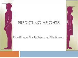
Predicting Heights Ryan Dickson, Dan Faulkner, and Bliss Brannon
The Task • We measured their height and our task is to predict the unknown teachers heights by creating a formula from out data. • We decided to measure the circumference of their bicep, the length of their upper arm, and the length from their knee to the floor.
Height vs. Knee to Floor Our r2 from our graph is 0.66, and our r is 0.812. Our graph is linear with a couple of outliers, is moderately strong, and the graph is positive. We have an outlier at (24,65). Our scatter plot is a good model because it is roughly linear when you remove the outlier. Also we have a strong correlation at 0.81 which means that the points on the graph are close to the LSR line and have small residuals. Our residual plot is a good model because it is scattered and does not seem to have a pattern
Female Height vs. Knee to Floor (difference in sex) • Males • The males generally had a longer knee to floor length, and their points had a stronger correlation. • Females • The females had a weaker correlation, and their knee to floor length was generally smaller than the males knee to floor length.
Height vs. Upper Arm Our r2 from the graph is 0.45, and our r is 0.671. The strength for our graph is moderate, and the graph is roughly linear. Our graph is positive with no outliers. Our scatter plot is a good model because it is roughly linear and it doesn’t have a weak correlation. The correlation is 0.671 which means that the LSR line is a good representation of our data. Our residual plot is a good model for this data because the graph is somewhat scattered. This means that all of the points are of almost equal distance from the line.
Height vs. Upper Arm (difference in sex) • Males • The correlation is 0.671, and their points were generally greater in height and upper arm length. • Females • The correlation is 0.616, and their points are mostly lower then the males with only a few being greater.
Height vs. Bicep Circumference Our r2is 0.30, and the r is 0.548. The graph for this data is moderately weak, and is barely linear with a positive correlation. There are a few outliers that aren't that great but they may be affecting the data. The scatter plot isn't the greatest model for the data because the correlation at 0.548 isn't that strong, and the graph is a bit scattered. The LSR does a good job of representing this data because the residual plot is scattered. Our residual plot is a good model for this data because the points on the graph are scattered. This means that the residual line goes through the center of the data.
Height vs. Bicep Circumference (difference in sex) • Males • The correlation for the males is 0.184. Their points are scattered which means that the LSR line does not fit this data very well. Their points are generally higher than the females. • Females • The correlation for the females is 0.272. Their points are more linear then the males but they are still scattered. The LSR line does not represent their data very well. Their points are generally lower than the males.
Best Model Our best model in predicting unknown heights is our scatter plot including the” knee to floor” vs. “height” variables. We chose this model to be the best because the scatter plot has the strongest correlation which is .812. This means that the data has a moderately strong linear relationship. If we eliminate the one outlier, you can see that the data hugs the LSR line. The residual plot is also the most scattered showing no signs of any apparent patterns.
Bias and Error Bias and error definitely played a factor in attaining our data. Before we started measuring our classmates, we discussed on the technique of how we were going to record each of the three quantitative measurements. An error that could have occurred is if any of the three researchers disregarded the technique on any of the 50 subjects. Also, we could have instinctively estimated the measurements to make the data easier upon ourselves. Some errors that the subjects could have contributed consist of • Not flexing completely when we measured their bicep • Not making the knee go straight down to the floor at a 90o angle • Subjects that didn’t stand up straight as we recorded their heights.
Group Member Predictions • Ryan • Predicted height 67.55 inch, actual height is 70 inch • Residual is 2.45 inch • Dan • Predicted 65.3 inch, actual height is 65.5 inch • Residual is .2 inch • Bliss • Predicted 73.175 inch, actual height is 75 inch • Residual is 1.825 inch
Teachers Predictions • Mrs. Arden • Predicted height is 66.425 inches • Mrs. Wilson • Predicted height is 65.3 inches • Mr. Smith • Predicted height is 69.8 inches • Mrs. Robinson • Predicted height is 70.925 inches
Conclusion We are confident in our predictions for the teachers heights because when we estimated our heights they were very close. Because of this we feel that our predictions for the teachers will be of by at most 2 inches. Overall we were satisfied with our results and we feel that we found a good model for predicting people’s heights.