Download
1 / 21
210 likes | 432 Vues
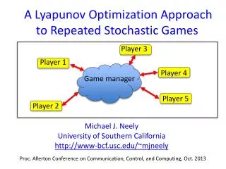
A Lyapunov Optimization Approach to Repeated Stochastic Games. Player 3. Player 1. Player 4. Game manager. Player 5. Player 2. Michael J. Neely University of Southern California http://www-bcf.usc.edu/~mjneely.

E N D
A Lyapunov Optimization Approach to Repeated Stochastic Games Player 3 Player 1 Player 4 Game manager Player 5 Player 2 Michael J. Neely University of Southern California http://www-bcf.usc.edu/~mjneely Proc. Allerton Conference on Communication, Control, and Computing, Oct. 2013
Game structure • Slotted time t in {0, 1, 2, …}. • N players, 1 game manager. • Slot t utility for each player depends on: • (i) Random events ω(t) = (ω0(t), ω1(t),…,ωN(t)) • (ii) Control actions α(t) = (α1(t), … , αN(t)) • Players Maximize time average utility. • Game manager • Provides suggestions. • Maintains fairness of utilities • subject to equilibrium constraints.
Random events ω(t) Player 1 ω1(t) Player 3 ω3(t) Game manager (ω0(t), ω1(t), …, ωΝ(t)) Player 2 ω2(t) • Player i sees ωi(t). • Manager sees: ω(t) = (ω0(t), ω1(t), … , ωN(t)) Only known to manager!
Random events ω(t) Player 1 ω1(t) Player 3 ω3(t) Game manager (ω0(t), ω1(t), …, ωΝ(t)) Player 2 ω2(t) • Player i sees ωi(t). • Manager sees: ω(t) = (ω0(t), ω1(t), … , ωN(t)) • Vector ω(t) is i.i.d. over slots • (components are possibly correlated)
Actions and utilities Player 1 α1(t) Player 3 α3(t) M3(t) M1(t) Game manager (ω0(t), ω1(t), …, ωΝ(t)) Player 2 α2(t) M2(t) • Manager sends suggested actions Mi(t). • Players take actions αi(t) in Ai. • Ui(t) = ui( α(t), ω(t) ).
Example: Wireless MAC game C1(t) User 1 Access Point C2(t) C3(t) User 2 User 3 • Manager knows current channel conditions: • ω0(t) = (C1(t), C2(t), … , CN(t)) • Users do not have this knowledge: • ωi(t) = NULL
Example: Economic market Player 1 Player 3 Game manager ω0(t) = [priceHAM(t)] [priceEGGS(t)] Player 2 • ω0(t) = vector of current prices. • Prices are commonly known to everyone: • ωi(t) = ω0(t) for all i.
Participation • At beginning of game, players choose either: • (i) Participate: • Receive messages Mi(t). • Always choose αi(t) = Mi(t). • (ii) Do not participate: • Do not receive messagesMi(t). • Can choose αi(t) however they like. Need incentives for participation…
Participation • At beginning of game, players choose either: • (i) Participate: • Receive messages Mi(t). • Always choose αi(t) = Mi(t). • (ii) Do not participate: • Do not receive messagesMi(t). • Can choose αi(t) however they like. • Need incentives for participation… • Nash equilibrium (NE) • Correlated equilibrium (CE) • Coarse Correlated Equilibrium (CCE)
ΝΕ for Static Game • Consider special case with no ω(t) process. • Nash equilibrium (NE): • Players actions are independent: • Pr[α] = Pr[α1]Pr[α2]…Pr[αN] • Game manager not needed. • Definition: • Distribution Pr[α] is a Nash equilibrium (NE) • if no player can benefit by unilaterally changing • its action probabilities. • Finding a NE in a general game is a nonconvex problem!
CΕ for Static Game • Manager suggests actions α(t) i.i.d. Pr[α]. • Suppose all players participate. • Definition: [Aumann 1974, 1987] • Distribution Pr[α] is a Correlated Equilibrium (CE) if: • E[ Ui(t)| αi(t)=α ] ≥ E[ ui(β, α{-i}) | αi(t)=α] • for all i in {1, …, N}, all pairs α, β in Ai. LP with |A1|2 + |A2|2 + … + |AN|2 constraints
Criticism of CE • Manager gives suggestions Mi(t)to players even if they do not participate. • Without knowing message Mi(t) = αi: • Player i only knows a-priori likelihood of other • player actions via joint distribution Pr[α]. • Knowing Mi(t) = αi: • Player i knows a-posteriori likelihood of other • player actions via conditional distribution Pr[α| αi]
CCΕ for Static Game • Manager suggests α(t) i.i.d. Pr[α]. • Gives suggestions only to participating players. • Suppose all players participate. • Definition:[Moulin and Vial, 1978] • Distribution Pr[α] is aCoarse Corr. Eq. (CCE)if: • E[ Ui(t) ] ≥ E[ ui(β, α{-i}) ] • for all i in {1, …, N}, all pairs β in Ai. LP with |A1| + |A2| + … + |AN| constraints. ( significantly less complex! )
Superset Theorem The NE, CE, CCE definitions extend easily to the stochastic game. Theorem: {all NE} {all CE} {all CCE}
Example (static game) Player 2 Player 2 2 5 50 1 4 2 2 4 Player 1 Player 1 3 5 3 0 Utility function 1 Utility function 2 (3.5, 2.4) All players benefit if non-participants are denied access to the suggestions of the game manager. CCE region Avg. Utility 2 NE and CE point (3.5, 9.3) (3.87, 3.79) Avg. Utility 1
Pure strategies for stochastic games • Player i observes: ωi(t)in Ωi • Player i chooses: αi(t) in Ai • Definition: A pure strategy for player i is a function bi: Ωi Ai. • There are |Ai||Ωi| pure strategies for player i. • Define Si as this set of pure strategies. Ωi Ai bi(ωi)
Stochastic optimization problem • φ( U1, U2, …, UN) Maximize: Concave fairness function CCE Constraints Subject to: 1) Ui≥Ui(s) for all iin {1, …, N} for all s in Si α(t) in A1 x A2 x … x AN for all t in {0, 1, 2, …} 2)
Lyapunov optimization approach Constraints: Virtual queue: Ui ≥ Ui(s) for all i in {1, …, N}, for all s in Si ui(s)(α(t), ω(t)) ui(α(t), ω(t)) Qi(s)(t) Formally: ui(s)(α(t), ω(t)) = ui((bi(s)(ωi(t)), α{-i}(t)), ω(t))
Online algorithm (main part): • Every slot t: • Game manager observes queues and ω(t). • Chooses α(t) in A1 x A2 x … x ANto minimize: • Do an auxiliary variable selection (omitted here). • Update virtual queues. • Knowledge of Pr[ω(t) = (ω0, ω1, …., ωN)] not required!
Conclusions: • CCE constraints are simpler and lead to improved utilities. • Online algorithm for the stochastic game. • No knowledge of Pr[ω(t) = (ω0, ω1, …., ωN)] required! • Complexity and convergence time is independent of size of Ω0. • Scales gracefully with large N.
Aux variable update: • Choose xi(t) in [0, 1] to maximize: • Vφ(x1(t), …, xN(t)) –∑Zi(t)xi(t) • Where Zi(t) is another virtual queue, one for each player i in {1, …, N}. See paper for details: • http://ee.usc.edu/stochastic-nets/docs/repeated-games-maxweight.pdf