Download
1 / 56
560 likes | 705 Vues
Use of Partial Orders for Analysis and Synthesis of Asynchronous Circuits. Alex Yakovlev School of EECE University of Newcastle upon Tyne. Collaboration with A. Semenov,W. Vogler, A. Kondratyev, V. Khomenko, M. Koutny, A. Madalinski, I. Poliakov. Outline. Motivation A bit of history

E N D
Use of Partial Orders for Analysis and Synthesis of Asynchronous Circuits Alex Yakovlev School of EECE University of Newcastle upon Tyne Collaboration with A. Semenov,W. Vogler, A. Kondratyev, V. Khomenko, M. Koutny, A. Madalinski, I. Poliakov
Outline • Motivation • A bit of history • Circuit models in Petri nets • Properties to be checked • Problems with unfolding models • State Coding analysis • Visualisation using unfoldings • Deriving logic from unfoldings • What next?
Motivation for asynchronous systems • Asynchronous (self-timed) systems help variability-tolerant design and optimize power-performance tradeoff for nanometer technology • Latest International Semiconductor Roadmap predicts 20% (40%) of designs will be asynchronous, and by 2012 (2020) • Active areas of asynchronous signalling and circuits: low power and low EMI processing (automotive, smart-card), networks on chip, GALS
Motivation from circuit analysis • Self-timed circuits can be highly concurrent, e.g. use of pipeline data flow structures, use of parallel branches in control of CPUs, concurrent resource allocation schemes (multi-way arbiters, switches etc.) – state space can run into 1030 for 100s of signals. Hence analysis and verification using explicit state space traversal is hard
Motivation from circuit synthesis • In the synthesis domain, resolving state encoding problems and constructing next-state functions using state space models is limited to 30-40 signals (relatively small controllers) • Visualisation of state space is very hard, let alone examining groups of states about some properties
A bit of history Early examples: • Flow chart, change chart methods by Gilles, Swartwout and Shelly – late 50s, early 60s • Signal Graphs for handshake control structures by Jump and Thiagarajan – mid 70s • Circuit synthesis from Taxograms by Starodoubtsev – mid 80s • Circuit analysis and synthesis using Change Diagrams and their unfoldings by Kishinevsky, Kondtayev, Taubin and Varshavsky – late 80s. • Relation-based approach to analysis of STG models by Rosenblum and Yakovlev – late 80s
A bit of history • Petri net unfolding prefix by McMillan (1992) • Unfolding prefix for STGs and circuits by Kondratyev et al. and Semenov (1995) • Unfolding-based analysis of Timed Circuits by Semenov and Yakovlev (1996) • Unfolding-based synthesis using cover approximations by Semenov et al. (1997) • Circuit analysis using contextual net unfoldings by Vogler et al. – (1998) • STG analysis using unfoldings and LP and SAT by Khomenko et al. (2002-2003) • Circuit Synthesis from STG using unfoldings and SAT by Khomenko (2004) • Visualization of STG-based Synthesis by unfoldings by Madalinski et al. (2003-2005) • Combining decomposition and unfolding for STG-based Synthesis by Khomenko and Shaefer (2007)
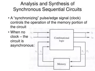
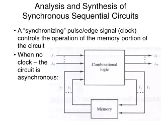
Circuit models in Petri nets • Event-based models: Petri net transitions represent signal events • Level-based models: Petri net places model the values of signals
Logic Circuit Modelling Event-driven elements Petri net equivalents C Muller C-element Toggle
Logic Circuit Modelling Level-driven elements Petri net equivalents y(=0) x=0 x(=1) y=1 y=0 x=1 NOT gate Read arcs x=0 x(=1) z(=0) z=1 y=0 y(=1) b NAND gate x=1 z=0 y=1
Circuit Petri Nets Level-driven elements Petri net equivalents Self-loops in ordinary P/T nets y(=0) x=0 x(=1) y=1 y=0 x=1 NOT gate x=0 x(=1) z(=0) z=1 y=0 y(=1) b NAND gate x=1 z=0 y=1
Logic Circuit Modelling: examples • Pipeline control must guarantee: • Handshake protocols between the stages • Safe propagation of the previous datum before the next one Pipeline data Stage Data Out Data In Data Enable Rin Rout Pipeline control Stage Ain Aout
Event-driven circuit Non-speed-independence can be detected via non-1-safeness check
Level-driven circuit Set-part
Level-driven circuit Reset-part
Without y2 in Set part of y1 this trace can happen: I2+ C1+ C2+ I2- I1+ C1- C2- I2+ C1+ Level-driven circuit This sort of structures (acyclic Change Diagrams) were built directly from logic eqn’s by Kishinevsky et al. – but only for distributive circuits
Level-driven circuit Without y2 in Set part of y1 this trace can happen: I2+ C1+ C2+ I2- I1+ C1- C2- I2+ C1+ disabling
Properties analysed • Functional correctness (need to model environment) • Deadlocks • Hazards: • non-1-safeness for event-based • non-persistency for level-based • Timing constraints • Absolute (need Timed Petri nets) • Relative (compose with a PN model of order conditions)
Circuit Petri Nets Level-driven elements Petri net equivalents Self-loops in ordinary P/T nets y(=0) x=0 x(=1) y=1 y=0 x=1 NOT gate x=0 x(=1) z(=0) z=1 y=0 y(=1) b NAND gate x=1 z=0 y=1
Unfolding Nets with Read Arcs Unfolding with read arcs PN with self-loops Unfolding with self-loops (work with W. Vogler, CONCUR 1998) Combinatorial explosion due to splitting the self-loops Works nicely for read-persistent nets only
Petri Net mapping: an example corresponding Petri Net source gate-level model Multiple read arcs exiting one place: bad for unfolding! Only one read arc per place:minimal impact on unfolding
STG Unfolding • Unfolding an interpreted Petri net, such as a Signal Transition Graph, requires keeping track of the interpretation – each transition is a change of state of a signal, hence each marking is associated with a binary state • The prefix of an STG must not only “cover” the STG in the Petri net (reachable markings) sense but must also be complete for analysing the implementability of the STG, namely: consistency, output-persistency and Complete State Coding
p1 a+ b+ p2 p3 c+ c+ p4 d+ p5 d- STG Unfolding STG Binary-coded STG Reach. Graph (State Graph) Uninterpreted PN Reachability Graph STG unfold. prefix p1 abcd p1 p1(0000) a+ b+ a+ b+ p3(0100) p2(1000) p2 p3 p2 p3 c+ c+ p4(0110) p4(1010) p4 c+ c+ d+ d+ p4 p4 p5(0111) p5(1011) p5 d+ d+ p5 p5 d- d-
p1 a+ b+ p2 p3 c+ c+ p4 d+ p5 d- STG Unfolding STG Binary-coded STG Reach. Graph (State Graph) Uninterpreted PN Reachability Graph STG unfold. prefix p1 abcd p1 p1(0000) a+ b+ a+ b+ p3(0100) p2(1000) p2 p3 p2 p3 c+ c+ p4(0110) p4(1010) p4 c+ c+ d+ d+ p4 p5(0111) p5(1011) p5 d+ Not like that! p5 d-
p1p6 b+ a+ b- p3p6 p2p6 Consistency and Signal Deadlock STG PN Reach. Graph STG State Graph p1 ab p1p6(00) b+ b+ a+ a+ b- p3p6(01) p2p6(10) p2 p3 a- a- b- p1p4(00) p1p4 b+ a+ b+ a- b- a+ b- b+ b+ p1p5(01) p2p4(10) p3p4 p3p4(01) p2p4 p1p5 p6 p4 b+ b+ b+ b+ b- Signal deadlock wrt b+ (coding consistency violation) p2p5(11) p2p5 p3p5 b+ b- b- b- b- p5
STG p1 b+ a+ p2 p3 a- b- p6 p4 b+ b- p5 Signal Deadlock and Autoconcurrency p6 p1 STG State Graph STG Prefix ab p1p6(00) b+ a+ b+ a+ b- p3p6(01) p3 p2p6(10) p2 a- b- a- b- p1p4(00) b+ p1 a+ b+ p4 p1p5(01) p2p4(10) p3p4(01) b+ b+ p2 b+ a+ Signal deadlock wrt b+ (coding consistency violation) p2p5(11) p5 b- b- p2 b- Autoconcurrency wrt b+
Verifying STG implementability • Consistency – by detecting signal deadlock via autoconcurrency between transitions labelled with the same signal (a* || a*, where a* is a+ or a-) • Output persistency – by detecting conflict relation between output signal transition a* and another signal transition b* • Complete State Coding is less trivial – requires special theory of binary covers on unfolding segments
Data Transceiver Device Bus d lds dsr VME Bus Controller ldtack dtack dtack- dsr+ lds+ d- lds- ldtack- ldtack+ dsr- dtack+ d+ Example: VME Bus Controller
10000 dtack- dsr+ 00100 00000 lds+ ldtack- ldtack- ldtack- dtack- dsr+ 10010 01100 01000 11000 ldtack+ lds- lds- lds- dtack- dsr+ 11010 01110 11010 M’’ M’ 01010 d+ d- dsr- dtack+ 01111 11111 11011 Example: Encoding Conflict
Example: Encoding Conflict e8 e10 dtack- dsr+ e1 e2 e3 e4 e5 e6 e7 e12 lds+ dsr+ lds+ ldtack+ dtack+ d+ dsr- d- Code(conf’)=10110 Code(conf’’)=10110 lds- ldtack- e9 e11
Detection of encoding conflicts using SAT solvers • A special case of model checking! • has the formCONF1CONF2VIOL • VIOLis a constraint stating that the two configurations have the same final encodings and enable different sets of output signals
Beyond model checking Problem: model checking just tells you whether some property holds, but it’s not enough for resolution of encoding conflicts and for deriving equations!
M’’ M’ Example: Resolving the conflict dtack- dsr+ csc+ 001000 100000 000000 100001 lds+ ldtack- ldtack- ldtack- dtack- dsr+ 011000 100101 010000 110000 ldtack+ lds- lds- lds- dtack- dsr+ 110101 011100 110100 010100 d+ d- dsr- dtack+ csc- 011111 111111 110111 011110
Example: Encoding Conflict e8 e10 core dtack- dsr+ e1 e2 e3 e4 e5 e6 e7 e12 lds+ dsr+ lds+ ldtack+ dtack+ d+ dsr- d- Code(conf’)=10110 Code(conf’’)=10110 lds- ldtack- e9 e11
dtack- dsr+ lds+ csc+ d- lds- ldtack- ldtack+ csc- dsr- dtack+ d+ Example: Resolving the conflict
Core1 Core2 Core3 A1 A2 A3 Visualising conflicts: Height map • Cores often overlap • Highest ‘peaks’ are good candidates for signal insertion • Analogy with topographic maps
Highest peak csc+ Height map: an example Core map Height map
Logic synthesis: Next-state function • Thenext-state functionof each output or internal signal will be implemented as a logic gate in the circuit • Defined for each such signalzat each reachable stateMas Nxtz(M) = Codez(M) Enabledz(M) • The value is undefined (‘don’t care’) for unreachable states
Example: Deriving equations dtack- dsr+ csc+ 001000 100000 000000 100001 lds+ ldtack- ldtack- ldtack- dtack- dsr+ 011000 100101 010000 110000 ldtack+ lds- lds- lds- dtack- dsr+ 110101 011100 110100 010100 d+ d- dsr- dtack+ csc- 011111 111111 110111 011110
Example: Resulting Circuit Data Transceiver Device Bus d lds dtack dsr csc ldtack
Logic synthesis on unfoldings Challenge: how to do this without building the state graph, and using only the unfolding prefix?
Logic synthesis on unfoldings • Problem:given a prefix and a setXof signals which are known to be a support of the given output or internal signalz,compute the truth table ofNxtz • Let = CONF CODEXwhere CODEXrelates the values of all signals inXwith the configuration • Compute the projection ofontoX Need to know how to compute projections!