CHAPTER 2 PROCESSOR SCHEDULING PART V
CHAPTER 2 PROCESSOR SCHEDULING PART V. by Uğur HALICI. 2.3.4 Round-Robin Scheduling (RRS). In RRS algorithm the ready queue is treated as a FIFO circular queue.


CHAPTER 2 PROCESSOR SCHEDULING PART V
E N D
Presentation Transcript
CHAPTER 2PROCESSOR SCHEDULINGPART V by Uğur HALICI
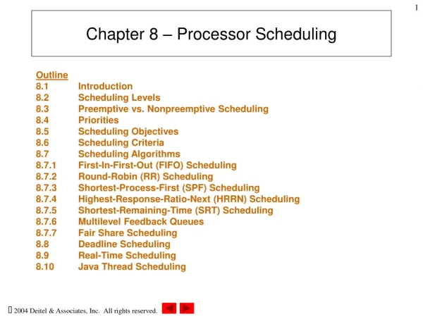
2.3.4 Round-Robin Scheduling (RRS) • In RRS algorithm the ready queue is treated as a FIFO circular queue. • The RRS traces the ready queue allocating the processor to each process for a time interval which is smaller than or equal to a predefined time called time quantum (slice).
2.3.4 Round-Robin Scheduling (RRS) • The OS using RRS, takes the first process from the ready queue, gives the processor to that process and sets a timer to interrupt when time quantum expires. • If the process has a processor burst time smaller than the time quantum, then it releases the processor voluntarily, either by terminating or by issuing an I/O request. • The OS then proceed with the next process in the ready queue.
2.3.4 Round-Robin Scheduling (RRS) • The performance of RRS depends heavily on the selected time quantum. • Time quantum RRS becomes FCFS • Time quantum 0 RRS becomes processor sharing (It acts as if each of the n processes has its own processor running at processor speed divided by n) • However, if time quantum is too small then context switch time can not be ignored anymore. • For an optimum time quantum, it can be selected to be greater than 80 % of processor bursts and to be greater than the context switching time.
2.3.4 Round-Robin Scheduling (RRS) RR Time quantum next_cpu_burst : remaining_time used FCFS
2.3.4 Round-Robin Scheduling (RRS) RR next_cpu_burst : remaining_time FCFS
2.3.4 Round-Robin Scheduling (RRS) expires preemption p
2.2 Process States If more than one processes are to enter the Ready Queue at the same time then give priority as: 1: process just submitted 2: process completed I/O 3: process preempted CPU preeemption 1 3 2 START READY HALTED RUNNING I/O completed I/O requested WAITING
2.3.4 Round-Robin Scheduling (RRS) expires preemption p p
2.3.4 Round-Robin Scheduling (RRS) expires p p
2.3.4 Round-Robin Scheduling (RRS) expires p p
2.3.4 Round-Robin Scheduling (RRS) expires p p
2.3.4 Round-Robin Scheduling (RRS) expires preemption p p p
2.3.4 Round-Robin Scheduling (RRS) expires p p p
2.3.4 Round-Robin Scheduling (RRS) expires p p p
2.3.4 Round-Robin Scheduling (RRS) expires p p p
2.3.4 Round-Robin Scheduling (RRS) expires p p p
2.3.4 Round-Robin Scheduling (RRS) expires p p p
2.3.4 Round-Robin Scheduling (RRS) expires preemption p p p p
2.3.4 Round-Robin Scheduling (RRS) expires p p p p
2.3.4 Round-Robin Scheduling (RRS) expires p p p p
2.3.4 Round-Robin Scheduling (RRS) expires preemption p p p p p
2.3.4 Round-Robin Scheduling (RRS) expires p p p p p
2.3.4 Round-Robin Scheduling (RRS) expires p p p p p
2.3.4 Round-Robin Scheduling (RRS) expires preemption p p p p p p
2.3.4 Round-Robin Scheduling (RRS) expires preemption p p p p p p p
2.3.4 Round-Robin Scheduling (RRS) expires p p p p p p p
2.3.4 Round-Robin Scheduling (RRS) expires p p p p p p p
2.3.4 Round-Robin Scheduling (RRS) • Processor utilization = (35 / 35) * 100 = 100 % • Throughput = 4 / 35 p p p p p p p
2.3.4 Round-Robin Scheduling (RRS) • Turn around time: tatA = 35 – 0 = 35 tatB = 34 – 2 = 32 tatC = 15 – 3 =12 tatD = 26 – 7 = 19 tatAVG = (35 + 32 + 12 + 19) / 4 = 24. p p p p p p p
2.3.4 Round-Robin Scheduling (RRS) • Turn around time: tatA = 35 – 0 = 35 tatB = 34 – 2 = 32 tatC = 15 – 3 =12 tatD = 26 – 7 = 19 tatAVG = (35 + 32 + 12 + 19) / 4 = 24. p p p p p p p
2.3.4 Round-Robin Scheduling (RRS) • Turn around time: tatA = 35 – 0 = 35 tatB = 34 – 2 = 32 tatC = 15 – 3 =12 tatD = 26 – 7 = 19 tatAVG = (35 + 32 + 12 + 19) / 4 = 24. p p p p p p p
2.3.4 Round-Robin Scheduling (RRS) • Turn around time: tatA = 35 – 0 = 35 tatB = 34 – 2 = 32 tatC = 15 – 3 =12 tatD = 26 – 7 = 19 tatAVG = (35 + 32 + 12 + 19) / 4 = 24. p p p p p p p
2.3.4 Round-Robin Scheduling (RRS) • Turn around time: tatA = 35 – 0 = 35 tatB = 34 – 2 = 32 tatC = 15 – 3 =12 tatD = 26 – 7 = 19 tatAVG = (35 + 32 + 12 + 19) / 4 = 24 p p p p p p p
2.3.4 Round-Robin Scheduling (RRS) • Waiting time: wtA = (0 – 0)+(8 – 3)+(17 – 13)+(24 – 20)+(29 – 29)+(34 – 32)=15 wtB = (3 – 2)+(9 – 6)+ (15 -12)+(21 – 18)+(26 – 24)+(32 – 29) =15 wtC = (6 – 3) + (13 – 9) = 7 wtD = (12 – 7) + (20 – 14) + (25 – 22) = 14 wtAVG = (15 + 12 + 7 + 11) / 4 = 11.25 p p p p p p p
2.3.4 Round-Robin Scheduling (RRS) • Waiting time: wtA = (0 – 0)+(8 – 3)+(17 – 13)+(24 – 20)+(29 – 29)+(34 – 32)=15 wtB = (3 – 2)+(9 – 6)+ (15 -12)+(21 – 18)+(26 – 24)+(32 – 29) =15 wtC = (6 – 3) + (13 – 9) = 7 wtD = (12 – 7) + (20 – 14) + (25 – 22) = 14 wtAVG = (15 + 12 + 7 + 11) / 4 = 11.25 p p p p p p p
2.3.4 Round-Robin Scheduling (RRS) • Waiting time: wtA = (0 – 0)+(8 – 3)+(17 – 13)+(24 – 20)+(29 – 29)+(34 – 32)=15 wtB = (3 – 2)+(9 – 6)+ (15 -12)+(21 – 18)+(26 – 24)+(32 – 29) =15 wtC = (6 – 3) + (13 – 9) = 7 wtD = (12 – 7) + (20 – 14) + (25 – 22) = 14 wtAVG = (15 + 12 + 7 + 11) / 4 = 11.25 p p p p p p p
2.3.4 Round-Robin Scheduling (RRS) • Waiting time: wtA = (0 – 0)+(8 – 3)+(17 – 13)+(24 – 20)+(29 – 29)+(34 – 32)=15 wtB = (3 – 2)+(9 – 6)+ (15 -12)+(21 – 18)+(26 – 24)+(32 – 29) =15 wtC = (6 – 3) + (13 – 9) = 7 wtD = (12 – 7) + (20 – 14) + (25 – 22) = 14 wtAVG = (15 + 12 + 7 + 11) / 4 = 11.25 p p p p p p p
2.3.4 Round-Robin Scheduling (RRS) • Waiting time: wtA = (0 – 0)+(8 – 3)+(17 – 13)+(24 – 20)+(29 – 29)+(34 – 32)=15 wtB = (3 – 2)+(9 – 6)+ (15 -12)+(21 – 18)+(26 – 24)+(32 – 29) =15 wtC = (6 – 3) + (13 – 9) = 7 wtD = (12 – 7) + (20 – 14) + (25 – 22) = 14 wtAVG = (15 + 12 + 7 + 11) / 4 = 11.25 p p p p p p p
2.3.4 Round-Robin Scheduling (RRS) • Response time: rtA = 0 – 0 = 0 rtB = 36 – 2 = 1 rtC = 6 – 3 = 3 rtD = 12 – 7 = 5 rtAVG = (0 + 1 + 3 + 5) / 4 = 2.25 p p p p p p p
2.3.4 Round-Robin Scheduling (RRS) • Response time: rtA = 0 – 0 = 0 rtB = 3 – 2 = 1 rtC = 6 – 3 = 3 rtD = 12 – 7 = 5 rtAVG = (0 + 1 + 3 + 5) / 4 = 2.25 p p p p p p p
2.3.4 Round-Robin Scheduling (RRS) • Response time: rtA = 0 – 0 = 0 rtB = 36 – 2 = 1 rtC = 6 – 3 = 3 rtD = 12 – 7 = 5 rtAVG = (0 + 1 + 3 + 5) / 4 = 2.25 p p p p p p p
2.3.4 Round-Robin Scheduling (RRS) • Response time: rtA = 0 – 0 = 0 rtB = 36 – 2 = 1 rtC = 6 – 3 = 3 rtD = 12 – 7 = 5 rtAVG = (0 + 1 + 3 + 5) / 4 = 2.25 p p p p p p p
2.3.4 Round-Robin Scheduling (RRS) • Response time: rtA = 0 – 0 = 0 rtB = 3 – 2 = 1 rtC = 6 – 3 = 3 rtD = 12 – 7 = 5 rtAVG = (0 + 1 + 3 + 5) / 4 = 2.25 p p p p p p p
2.3.4 Round-Robin Scheduling (RRS) • In Round Robin Scheduling it is guaranteed that rtmax≤ (n-1)*Q where n : multiprogramming degree Q: time quantum
2.3.5 Priority Scheduling • In this type of algorithms a priority is associated with each process and the processor is given to the process with the highest priority. Equal priority processes are scheduled with FCFS method. • To illustrate, SPF is a special case of priority scheduling algorithm where Priority(i) = 1 / next processor burst time of process i or Priority(i) = K - next processor burst time of process i
2.3.5 Priority Scheduling • Priorities can be fixed externally or they may be calculated by the OS from time to time. • Externally, if all users have to code time limits and maximum memory for their programs, priorities are known before execution. • Internally, a next processor burst time prediction such as that of SPF can be used to determine priorities dynamically.
2.3.5 Priority Scheduling • A priority scheduling algorithm can leave some low-priority processes in the ready queue indefinitely. • If the system is heavily loaded, it is a great probability that there is a higher-priority process to grab the processor. • This is called the starvation problem. • One solution for the starvation problem might be to gradually increase the priority of processes that stay in the system for a long time.
2.3.5 Priority Scheduling Example: Following may be used as a priority defining function: Priority (i) = 10 + tnow – ts(i) – trq(i) – tcpu(i) Where ts(i): the time process n is submitted to the system Trq(i): the time process n entered to the ready queue last time Tcpu(i): next processor burst length of process n tnow:current time • P(i)=tnow – trq(i)≈FCFS • P(i)=K– tcpu(i)≈SPF • P(i)=α(tnow – trq(i))+(1-α)(K– tcpu(i)), ≈combination of FCFS & SPF