Download
1 / 59
590 likes | 696 Vues
University of. Maryland. IRT Models to Assess Change Across Repeated Measurements. James S. Roberts Georgia Institute of Technology Qianli Ma University of Maryland. Many Thanks!!!. Thanks Bob.

E N D
University of Maryland IRT Models to Assess Change Across Repeated Measurements James S. Roberts Georgia Institute of Technology Qianli Ma University of Maryland
Many Thanks!!! • Thanks Bob. • Thanks to Mayank Seksaria,Vallerie Ellis, Dan Graham, Yi Cao, and Yunyun Dai for their assistance at various stages of this project. • Thanks to the Project MATCH Coordinating Center at the University of Connecticut for sharing their data.
Situations in Which Repeated Measures IRT Models Are Useful • Each respondent receives the same test multiple times • Typical pretest, posttest, follow-up, treatment studies • Each respondent receives alternate forms of a comparable test with common items across forms (or across pairs of forms) • More elaborate repeated measures designs that control for memory effects
Each respondent receives alternate forms that are not comparable (in difficulty) but have some common items • Vertical measurement situations • ECLS, Some school testing programs • Each of these situations involves a set of common items across (successive pairs of) administered tests • 100% common items = same form • Less than 100% common items = alternate forms
Typical Approaches to Repeated Measures Data In IRT • Calibrate responses from each administration separately • Ignores correlation of the latent trait across test administrations • Calibrate responses from each administration simultaneously allowing for different prior distributions at each administration • Still ignores correlation
Multidimensional Approaches • Andersen (1985) • Reckase and Martineau (2004) • Estimate theta at each testing occasion simultaneously • Does incorporate correlation across testing occasions • Does not really assess change in the latent variable
An Alternative IRT Approach • Embretson’s (1991) Multidimensional Rasch Model for Learning and Change (MRMLC) • Developed to measure change in a latent trait across repeatedly measured items that are scored as binary variables
Where: is the baseline (time 1) level of the latent trait for the jth respondent is the change in the level of latent trait from time1 to time 2 for the jth respondent is the change in the level of latent trait from time t -1 to time t for the jth respondent with t = 2, …, T
bi(t) is the difficulty of the ith item nested within test administration t There must be common items across test form administrations and the difficulty is assumed constant for a given common item This maintains the metric across forms
This model parameterizes the latent trait scores for each individual as an initial trait level followed by t-1 latent change scores • It is multivariate in the sense that each individual has T latent trait scores • However, each of these scores relates to positions on a single unidimensional continuum
Note that: So the latent trait level for the jth individual at time t (i.e., the composite trait at time t ) is the sum of the initial level along with all the latent change scores
Along with estimates of the aforementioned parameters, one also obtains estimates of the latent variable means and the correlation matrix for these latent variables:
Advantages of the Multidimensional IRT Approach to Change • Traditional Benefits of IRT Models that Fit the Data • Sample invariant interpretation of item parameters • Item invariant interpretation of person parameters • Index of precision at the individual level
Advantages to measuring change with this multidimensional IRT approach • Parameterizing change as an additional dimension in an IRT model eliminates the reliability paradox associated with observed change scores classical test theory • Higher correlation between pretest and posttest lead to less reliable observed change scores • The precision of IRT measures of latent change do not depend on pretest to posttest correlations
Small changes in observed scores may have a different meaning when the initial observed score is extreme rather than more moderate • Because the relationship between the expected test score and the latent trait is nonlinear, an IRT model allows for this relationship
Further Generalization of the Basic Model • One can easily extend the MRMLC to more general situations • Allow for graded (polytomous) responses Wang, Wilson & Adams (1998) Wang & Chyi-In (2004)
We have generalized the basic model further in this project by allowing items to vary in their discrimination capability • Form a similar model of change using Muraki’s (1991) generalized partial credit model
Where: is the baseline level of the latent trait for the jth respondent is the change in the level of latent trait from baseline to time 2 for the jth respondent is the change in the level of latent trait from time t -1 to time t for the jth respondent with t = 2, …, T
bi ( t ) k is the kth step difficulty parameter for the ith item on the test administration t ai ( t ) is the discrimination parameter for the ith item on test administration t Again, these item parameters are held constant for common items on successive test administrations.
Example 1: Beck Depression Inventory • 21 self-report items designed to measure depression • Two items were clearly not appropriate for a cumulative IRT model • Appetite loss and weight loss
Remaining items relate to: • Sadness, discouragement, failure, dissatisfaction, guilt persecution, disappointment, blame, suicide, crying, irritation, interest in others, decisiveness, attractiveness appraisal, ability to work, ability to sleep, tiring, worry, sexual interest • Four response categories per item • Graded item responses coded as 0 to 3 • Higher item scores are indicative of more severe symptoms
1322 subjects in an alcohol treatment clinical trial • Responses from Baseline, End of 3 month alcoholism treatment period, and 9-month follow-up
Dimensionality Assessment Eigenvalue Ratio Baseline 7.01 / 1.32 3-Months 7.72 / 1.23 9-Months 7.83 / 1.39
Classical Test Theory Statistics Baseline Mean Score: 9.52 s.d. 7.94 a=.90 3 Months Mean Score: 6.75 s.d. 7.29 a=.90 9 Months Mean Score: 6.94 s.d. 7.45 a=.91
Classical Test Theory Statistics (cont.) ITC ___ ___ Time Range Obs. Obs. range Baseline (.34, .64) .50 (.12, .76) 3 Months (.20, .72) .36 (.11, .53) 9 Months (.36, .71) .37 (.13, .53)
Classification Baseline 3 Mo. 9 Mo. No Depression 56.2% 71.4% 69.1% Mild 29.5% 19.7% 20.9% Moderate 10.8% 6.3% 7.9% Severe 3.5% 2.6% 2.1%
Parameter Estimation • Markov Chain Monte Carlo estimation with WinBUGS MVN(m, S) prior for N(0,4) prior for LN(0,.25) prior for Estimation requires two constraints on a common item Set one step difficulty parameter and one discrimination parameter to constant values
Item Parameter Estimates Range Mean b. (1.37, 2.38) 1.82 a (.43, 2.73) 1.62
Estimated Person Distribution Hyperparameters Baseline .362 .861 Change from -.525 .856 Baseline to Tx End (3 Months) Change from Tx .002 .829 End to Follow-up (3 to 9 Months)
Example 2: Simulated Multiple Forms Design • Two Assessment Periods With a 20-Item Form Administered at Each Testing Period • Four items are common across test forms • Item parameters sampled from 3-category items from the 1998 NAEP Technical Report
True Item Parameters Form 1 Form 2 b. Range (-1.01, 1.74) (-1.01, 1.70) b. Mean .11 .50 a Range (.56, 1.23) (.56, 1.57) a Mean .90 1.00
Person Parameters at Time 1 and Change at Time 2 were Sampled From a Bivariate Normal Distribution with r = -.243 qj1* ~ N(0, 1) qj2* ~ N(.5, 1.0625) • 2000 Simulees
Estimated Item Parameters Range Mean Form 1 Form 2 Form 1 Form 2 b. ( -.99, 1.74) ( -.99, 1.87) .17 .61 (-1.01, 1.74) (-1.01, 1.70) .11 .50 a (.53, 1.15) (.53, 1.43) .85 .96 (.56, 1.23) (.56, 1.57) .90 1.00
Estimated Person Distribution Hyperparameters Time 1 .07 1.08 .00 1.00 Change from .54 1.10 Time 1 to Time 2 .50 1.03