Download
1 / 33
370 likes | 719 Vues
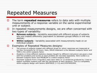
Repeated Measurements Analysis. Repeated Measures Analysis of Variance. Situations in which biologists would make repeated measurements on same individual Change in a trait or variable measured at different times E.g., clutch size variation over time

E N D
Repeated Measures Analysis of Variance • Situations in which biologists would make repeated measurements on same individual • Change in a trait or variable measured at different times • E.g., clutch size variation over time • Change in survivorship over time among populations • Individual is exposed to different level of a same treatment • E.g., same plants exposed to varying [CO2]
Response Time
How to Analyze Repeated Measures Designs • Univariate and Multivariate Approaches • Univariate • Randomized Designs • Split-plot designs • Multivariate: • MANOVA • Mixed Model Analysis • GLMM (General Linear Mixed Model) • Non-linear analysis (counts) • Mixed Model Approach is preferred method
Advantages of Repeated Measures • Recall that experimental design has goal of reducing error and minimizing bias • E.g., use randomized blocks • In repeated measures individuals are “blocks” • Assume within-subject variation lower than among subjects • Advantage – can conduct complex designs with fewer experimental units
Concepts Continued All repeated measures experiments are factorial Treatmentis called the between-subjectsfactor levels change only between treatments measurements on same subject represent same treatment Time is called within-subjectsfactor different measurements on same subject occur at different times
Hypotheses • How does the treatment mean change over time? • How do treatment differences change over time?
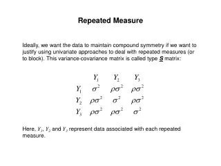
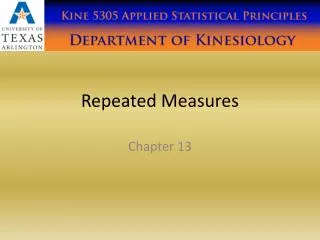
Why is Repeated Measures ANOVA unique? • Problem involves the covariance structure • Particularly the error variance covariance structure • ANOVA and MANOVA assume independent errors • All observations are equally correlated • However, in repeated measures design, adjacent observations are likely to be more correlated than more distant observations
1.0 0.0 Lag Time
Basic Repeated Measures Design • Completely Randomized Design (CRD) • Data collected in a sequence of evenly spaced points in time • Treatments are assigned to experimental units • I.e., subjects • Two factors: • Treatment • Time
Overview of Univariate Approaches • Based on CRD or split-plot designs • Hypothesis: do different treatment levels applied to same individuals have a significant effect • CRD: Individual is the block • Blocking increases the precision of the experiment • Measurements made on different time periods comprise the within-subject factor
Univariate Approach • Split-Plot Design: • Treatment factor corresponds to main-plot factor • I.e., between-subjects factor is main plot factor • Time factor is the sub-plot factor • I.e., within-subjects is the sub-plot factor • Problem: in true split-plot design • Levels of sub-plot factor are randomly assigned • Equal correlation among responses in sub-plot unit • Not true in repeated measures design – measurements made at adjacent times are more correlated with one another than more distant measurements
Univariate Approach • Assumptions must be made regarding the covariance structure for the within-subject factor • Circularity • Circular covariance matrix: difference between any two levels of within-subject factor has same constant value • Compound Symmetry • All variances are assumed to be equal • All covariances are assumed to be equal • Sphericity may be used to assess the circularity of covariance matrix • One must test for these assumptions otherwise F-ratios are biased
Test of Assumptions: Univariate Approach • Sphericity and Compound Symmetry • Mauchley’s Test for Sphericity • Box (1954) found that F-ratio is positively biased when sphericity assumption is not met • Tend to reject falsely • How far does covariance matrix deviate from sphericity? • Measured by • If sphericity is met, then = 1 • Adjustments for positive bias (degrees of freedom): • Greenhouse-Geiser (Very conservative adjustment) • Huynh-Feldt condition(Better to estimate and adjust df with the estimated .)
(a) Variances at each time point (visually) Does variance look equal across time points? Looks like most variability is at Time1 and least at Time 4.
MANOVA Approach • Successive response measurements made over time are considered correlated dependent variables • That is, response variables for each level of within-subject factor is presumed to be a different dependent variable • MANOVA assumes there is an unstructured covariance matrix for dependent variables • Entails using Profile Analysis
Concerns using MANOVA • Sample size requirements • N – M > k • I.e., the number of samples (subjects) (N) less the number of between-subjects treatment levels (groups)(M) must be greater than the number of dependent variables • Low sample sizes have low power • Power increases as ratio n:k increases • May have to increase N and reduce k to obtain reasonable analysis using MANOVA
What does MANOVA test • Performs a simultaneous analysis of response curves • Evaluates differences in shapes of response curves • Evaluates differences in levels of response curves • Based on profile analysis – combines multivariate and univariate approaches
Profile Analysis • Test that lines are parallel • Test of lines equal elevation • Test that lines are flat
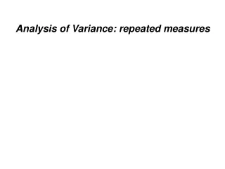
Cholesterol Level (mg/dl) treatment placebo 12 10 0 6 8 2 4 TIME (months) Profile Plots Illustrating the Questions of Interest TIME EFFECT ONLY Cholesterol Levels for both groups decreased over TIME however the decrease appears to be the same for both treatment groups, i.e. there is NO TREATMENT effect nor a TIME*TREATMENT interaction.
Cholesterol Level (mg/dl) treatment placebo 12 10 0 6 8 2 4 TIME (months) Profile Plots Illustrating the Questions of Interest TIME and TREATMENT EFFECT Cholesterol Levels for both groups decreased over TIME and the trend over time was the same for both groups, however the decrease for those receiving the drug was larger, i.e. there is a TREATMENT EFFECT.
Cholesterol Level (mg/dl) treatment placebo 12 10 0 6 8 2 4 TIME (months) Profile Plots Illustrating the Questions of Interest TIME*TREATMENT INTERACTION Here the effect of time is NOT the same for both groups. Thus we say that there is TIME and TREATMENT interaction.
Repeated Measures Analysis as a Mixed Model • Repeated measures analysis is a mixed model • Why? • First, we have a treatment, which is usually considered a fixed effect • Second, the subject factor is a random effect • Models with fixed and random effects are mixed models • A model with heterogeneous variances (more than one parameter in covariance matrix) is also a mixed model
Random Effects • Random-effects are factors where the levels of the factor in experiment are a random sample from a larger population of possible levels • Models in which all factors are random are random effects, or nested, or hierarchicalmodels
The mixed model • GLMM is defined as: • Y, X, and are as in GLM • Z is a known design matrix for the random effects • - vector of unknown random effects parameters • - vector of unobserved random errors • , are uncorrelated (assumption)
Why use Mixed Models to analyze Repeated Measure Designs? • Can estimate a number of different covariance structures • Key because each experiment may have different covariance structure • Need to know which covariance structure best fits the random variances and covariance of data • Missing values and Zeroes are not a problem here
Strategies for finding suitable covariance structures • Run unstructured first • Next run compound symmetry – simplest repeated measures structure • Next try other covariance structures that best fit the experimental design and biology of organism
Criteria for Selecting “best” Covariance Structure • Need to use model fitting statistics: • AIC – Akaike’s Information Criteria • SBC – Schwarz’s Bayesian Criteria • Larger the number the better • Usually negative so closest to 0 is best • Goal: covariance structure that is better than compound symmetry
Covariance Structures: Simple • Equal variances along main diagonal • Zero covariances along off diagonal • Variances constant and residuals independent across time. • The standard ANOVA model • Simple, because a single parameter is estimated: the pooled variance
Covariance Structures: Unstructured • Separate variances on diagonal • Separate covariances on off diagonal • Multivariate repeated measures • Most complex structure • Variance estimated for each time, covariance for each pair of times • Need to estimate 10 parameters • Leads to less precise parameter estimation (degrees of freedom problem)
Covariance Structures: compound symmetry • Equal variances on diagonal; equal covariances along off diagonal (equal correlation) • Simplest structure for fitting repeated measures • Split-plot in time analysis • Used for past 50 years • Requires estimation of 2 parameters
Covariance Structures: First order Autoregressive • Equal variances on main-diagonal • Off diagonal represents variance multiplied by the repeated measures coefficient raise to increasing powers as the observations become increasingly separated in time. Increasing power means decreasing covariances. Times must be equally ordered and equally spaced. • Estimates 2 parameters