Traffic Control

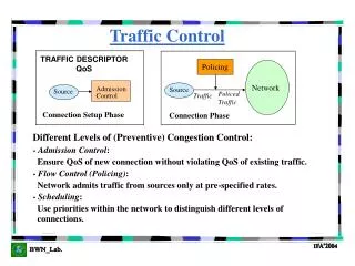
1. Policing Traffic Control TRAFFIC DESCRIPTOR QoS Network Admission Control Source Source Policed Traffic Traffic Connection Setup Phase Connection Phase Different Levels of (Preventive) Congestion Control: - Admission Control: Ensure QoS of new connection without violating QoS of existing traffic. - Flow Control (Policing): Network admits traffic from sources only at pre-specified rates. - Scheduling: Use priorities within the network to distinguish different levels of connections.

2. Traffic Descriptors(Specified for every connection) • Peak Cell Rate (PCR) = 1/T in units of cells/second, where T is the minimum intercell spacing in seconds, i.e., the time interval from the first bit of one cell to the first bit of the next cell. PCR is the minimum time interval between two consecutive cells. (T  1 sec) • Cell Delay Variation (CDV) Tolerance = t in seconds. The number of cells, B, that can be sent back-to-back at the access line is B =

3. Source Behavior Cell Interarrival Time CBR time Cell Interarrival Time Burst Duration Burst to Burst Interval VBR time Call Duration Call Tear-Down Call Set-up

4. Traffic Descriptors(Specified for every connection) • Peak Cell Rate (PCR): Max. amount of traffic that can be submitted by a source to an ATM network & expressed as ATM cells per second. Caveat: Peak bit rate of a source, (max. number of bits per second submitted to an ATM connection). PCR > Peak Bit Rate

5. Sustainable Cell Rate (SCR) is the maximum average rate that a bursty, on-off source traffic, can be sent at the peak rate.(Range: Lower Bound  Upper Bound Rates) Maximum Burst Size (MBS) is the maximum number of cells that can be sent at the peak rate. Traffic Descriptors (Specified for VBR Connections)

6. Calculate: The average # of cells submitted by the source over successive short periods of T. If the source transmits for a period of D=30 minutes and T=1 sec, then there are 1800 T periods and we will obtain 1800 averages, one per period. The largest of all these averages is called the SCR. Remark: SCR cannot be larger than PCR and be less than the Average Cell Rate. Remark: If we set T=D, then SCR becomes ACR at which the source submits cells to ATM. e.g., If T=30 min, then SCR=ACR.

7. Traffic Descriptors • Derived from collected statistics or from Network Operator’s • estimate of what is required. • The subscriber may not know in advance of what is required. • For new connection requests, the subscriber may not know in advance • the expected traffic behavior. • Thus, the user only specifies the type of service to be provided • in high-level terms (e.g., voice, video-telephony, or image database • browsing,) as well as QoS (e.g., image resolution – high, medium, or low). • Network providers are responsible for deriving the appropriate • traffic parameters and ensuring that the QoS requirements are achieved.

8. Peak Cell Transfer Rate: Minimum intercell arrival time between two consecutive cells • Connection Burst Rate: Minimum time allowed for the arrival of B cells, where B is the maximum expected burst length (e.g., video traffic); the max # of cells sent back to back. • Average Rate: Number of cells expected to arrive during a fairly long time period Example: Video: Peak RateAverage Rate (Mb/s) 11.75 3.0 14.42 4.2 44.7 16.8

9. Quality of Service (QoS) Expectations Applications have service requirements on: • - Throughput Output Rates = System Productivity • - Maximum Delay  End-to-End Delay • - Variance of Delays (Delay Jitter) • - Loss Probability  (e.g., BER= 10-12 ) • Network MUST guarantee the required Quality of Service (Traffic Contract)

10. QoS Parameters(Negotiated through Signaling) • Mean Cell Transfer Delay (Mean CDT) • Peak to Peak Cell Delay Variation (CDV) • Maximum Cell Transfer Delay (Max CDT) • Cell Loss Ratio (CLR) • Cell Error Rate (CER) = =

11. Severely Errored Cell Block Ratio (SECBR) • A cell block is a sequence of N cells transmitted consecutively on a given connection. A severely errored cell block outcome occurs when more than M errored cells, lost cells, or misinserted cells outcomes are observed in a received cell block. • Cell Misinsertion Rate (CMR) Cell misinsertion on a particular connection is most often caused by an undetected error in the header of a cell being transmitted on a different connection. This performance parameter is defined as a rate (rather than the ratio) since the mechanism producing misinserted cells is independent of the number of transmitted cells received on the corresponding connection.

12. Table of Procedures Used to Set Value of Traffic Contract Parameters Explicitly Specified Parameters Implicitly Specified Parameters Parameter Values set at Subscription Time by the Network Operator Parameter Values set at Connection-Setup Time Parameter Values set Using Default Rules Requested by Users/NMS Assigned by Network Operator SVC Network-operator default rules By subscription Signaling PVC Network-operator default rules By subscription NMS SVC = Switched Virtual Connection PVC = Permanent Virtual Connection NMS = Network Management System

13. Traffic Classes CBR: Constant Bit Rate rt-VBR: real-time Variable Bit Rate nrt-VBR: non-real-time Variable Bit Rate ABR: Available Bit Rate (Guarantee that the traffic will be transmitted by certain time) UBR: Unspecified Bit Rate (No guarantees!) Enhancement of UBR: GFR  Guaranteed Frame Rate

14. Traffic Classes GFR: (Undecided whether separate category or within UBR) Ensure minimum rate guarantees to UBR VCs. Rate guarantee is provided at frame level. GFR also guarantees fairness, i.e., share any capacity left behind fairly among the GFR VCs. Applications: Sources can neither specify the SCR and Burst Size needed for a VBR connection nor can be subject to ABR source rules (Minimum Cell Rate). PCR, MCR, MBS and Max Frame Size and CLR.

15. QoS Class QoS Parameters Application 0 1 2 3 4 Unspecified Specified Specified Specified Specified “Best Effort”, UBR Circuit Emulation, CBR VBR Video/Audio Connection-Oriented Data Connectionless Data QoS Classes:

16. Example Applications for CBR: • Interactive Video (e.g., videoconferencing) • Interactive Audio (e.g., telephone) • Video Distribution (e.g., television, distributed classroom) • Audio Distribution (e.g., radio, audio feed) • Video Retrieval (e.g., video-on-demand) • Any data/text/image transfer application which contains smooth enough traffic or for which the end-system’s response time requirements justify occupying a fully reserved CBR channel. • Example Applications for real-time (rt-VBR): • Any CBR application for which the end-system can benefit from statistical • multiplexing by sending at a variable rate, and can tolerate or recover from a • small but non-zero random loss ratio. • Any CBR application for which variable rate transmission allows more • efficient use of network resources. • Example Applications for non-real-time (nrt-VBR): • Response time critical transaction processing (e.g. airline reservations, • banking transactions, process monitoring) • Frame Relay interworking

17. Example Applications for UBR: • Interactive Text/Data/Image Transfer (e.g., banking transaction, credit card • verification) • Text/Data/Image Messaging (e.g., e-mail, telex, fax) • Text/Data/Image Distribution (e.g., news feed, weather sat. pictures) • Text/Data/Image Retrieval (e.g., file transfer, library browsing) • Aggregate LAN (e.g., LAN interconnection or emulation) • Remote Terminal (e.g., telecommuting, telnet) • Example Applications for ABR: • Any UBR application for which the end-system requires a guaranteed QoS. • Critical data transfer (e.g., defense information). • Super computer applications. • Data communication applications requiring better delay behavior, such as • remote procedure call, distributed file service (e.g., NFS), or computer process • swap/paging.

18. Example Applications for GFR: • For Heterogeneous (Hybrid) Networks, network elements outside ATM can benefit  i.e., IP routers could use GFR VCs to exchange control messages. • Current Internet applications are not designed to run over QoS-based networks. These applications could benefit from a minimum rate guarantee by the network, along with an opportunity to use the bandwidth fairly.

19. ATM Layer Service Categories Attribute CBR rt-VBR nrt-VBR UBR ABR specified specified PCR and CDVT specified 3 4 5 SCR, MBS n/a specified n/a 5,6 Min. Cell Rate MCR n/a n/a specified unspecified unspecified Peak-to-peak CDV specified specified unspecified unspecified unspecified Mean CDV unspecified unspecified specified Maximum CTD specified specified unspecified unspecified unspecified CLR unspecified specified specified 1 2 Feedback unspecified unspecified specified 7 Overview (Traffic & QOS Parameters)

20. Notes: 1. For CBR, rt-VBR, and nrt-VBR, the Cell Loss Ratio may be unspecified for CLP=1. 2. Minimized for sources that adjust cell flow in response to control information. 3. May not be subject to CAC and UPC procedures. 4. Represents the maximum rate at which the source can send as controlled by the control information. 5. These parameters are either explicitly or implicitly specified for PVCs or SVCs. 6. Different values of CDVT may be specified for SCR and PCR. 7. See Section on “ABR Flow Control”

21. Connection Admission Control (CAC) • The primary function of the CAC is to accept a new connection request only • if its stated QoS can be maintained without influencing the QoS of the already accepted connections. • It is very likely that certain calls will require more than one connection • (e.g., teleconferencing) CAC procedure must be performed for each requested • VCC or VPC. • CAC must • - Decide whether connections can be accepted or not. • - Provide parameters required by the UPC. • - Perform resource allocation.

22. Connection Admission Control (CAC) Typically, the decision to accept or reject a new connection is based on the answers to the following two questions: • Does the new connection affect the QoS of other existing connections? • Can the network provide the QoS expectations required by this new connection?

23. Request for VCC originates yes VPC exists Can QoS be satisfied? yes no no Establish a new VPC or VCC Block VCC or request more capacity Make connection Request granted yes no Reject VCC request Call Establishment Process Using Virtual Paths

24. Parameters demanded by the user which CAC uses, e.g.,: • Cell Loss Ratio (for data traffic, it is of the order of 10-12) • Cell Delays (for voice 500 ms round trip delay is noticeable) • Cell Delay Jitter (important for voice traffic and multiple streams 1ms) • (NOTE: For exact PARAMETER SPECS see the earlier explanation!!!) • Parameters of the source specified by the user which CAC uses, e.g.,: • Peak Rate of the Source • Sustainable Cell Rate of the Source • Maximum Burst Duration of the Source • (NOTE: See the exact PARAMETERS earlier!!!!) • Network statistics used by the CAC for making the decision: Available BW on each of the established or desired paths

25. Source Behavior Cell Interarrival Time CBR time Cell Interarrival Time Burst Duration Burst to Burst Interval VBR time Call Duration Call Tear-Down Call Set-up VBR Source Description: ON OFF Burst Length Distribution Interarrival Distribution During Burst Idle (Silent) Length Distribution Peak Cell Rate Sustainable Service Rate Mean Burst Length or < PCR, SCR, MBS >

26. Source Characterization Markovian Sources Long Range Dependency Processes (Self-Similar Processes) IBP On-Off MMPP IFP Voice, Video Traffic Markov Modulated Poisson Process Interrupted Fluid Process Interrupted Bernoulli Process Poisson Process Valid Data Traffic

27. Bandwidth Allocation Fixed Bandwidth Allocation(Guaranteed BW)(Peak BW Allocation) Dynamic Bandwidth Allocation

28. Bandwidth Allocation • PEAK BANDWIDTH ALLOCATION(DETERMINISTIC) • Suppose a source has an average BW of 20 Mbps and a peak BW of 45 Mbps. • Peak BW allocation requires that 45 Mbps be reserved at the output port for • the specific source independent of whether or not the source transmits • continuously at 45 Mbps. • Peak BW allocation is used for CBR services. • The new connection is accepted, if the sum of the peak rates of all the existing • connections plus the peak rate of the new connection is less than the capacity of • the output link. • ADVANTAGE: Easy to decide whether to accept a new connection or not. • DISADVANTAGE: Output port link will be underutilized if the sources do not • transmit at their peak rates. • STATISTICAL ALLOCATION(Dynamic Allocation) • The allocated BW is less than the peak rate of the source. • The sum of all peak rates may be greater than the capacity of the output link.

29. CBR, rt-VBR BW is allocated in deterministic fashion according to the peak rate Bandwidth Allocation (Cont.)

30. C1 C Trunk QoS   Cell Loss Probability Server Finite Buffer Dynamic BW Allocation Consider a single source feeding a finite capacity queue: Objective: Dynamic Bandwidth Allocation (Statistical)

31. Bandwidth Estimation • In order to allocate bandwidth, it needs to be estimated; • i.e., if a source with QoS expectations is admitted, will it • affect other already existing connections. BW Estimation Techniques Heavy Traffic Approximation Equivalent Capacity Link Metric Approach Upper Bounds of Cell Loss Probabilities Fast Buffer BW Allocation Time Windows (Stop & Go)

32. Equivalent Bandwidth(Link Metric Approach) Use Traffic Descriptors, Cell Loss Rate, and Buffer Size Traffic Sourceis defined by (r,,B) and has QoS requirements Q(D,e). r: Peak rate of the source : Ratio of the average rate to peak rate of the source B: Maximum burst length D: Delay requirement e: Required error bound (CELL LOSSES) for the source

33. C: Link Capacity x = D · C Source C The maximum number of sources that can be multiplexed onto the link without violating QoS: Easy to enforce Call Admission Process Test whether the sum of all equivalent BWs is less than or equal to available BW.

34. Factors Equivalent Bandwidth depends on: Ratio of the peak rate of the call to the link rate Burstiness: the factor  as shown above determines this. In the above expression, as  becomes 0, the total bandwidth required then = r/2-D·C/(2B). Burst Lengths: As the burst length increases, the equivalent bandwidth also increases.

35. Here, it is assumed that all sources have the same QoS requirements. • Inaccuracies because: • Fluid Flow Approximation used to derive is insensitive to stochastic structure of source behavior. • Assumed that equivalent bandwidth is not dependent on the already admitted sources. Overestimation of the required bandwidth possible. • Focuses on the Cell Loss Probability as the only QoS parameter. Uses it as an upper bound.

36. Demultiplexing Entering Cross Traffic Multiplexing Entering Cross Traffic Entering Cross Traffic Departing Cross Traffic Departing Cross Traffic Departing Cross Traffic End-To-End Model Used By CAC CAC is based on an abstract performance model of the network. - FINITE BUFFERS - DETERMINISTIC SERVICE TIMES Modeling Problems Need for accurate end-to-end queuing models because : - Because arrival streams (non-Poisson traffic) - Finite buffers at the multiplexers and switches - Correlated cell arrivals - Large state-space of the resulting system - Simulations of such systems take very long to converge

37. Policing (Usage Paramer Control (UPC)) • The operation of the CAC and the correct allocation of resources depend heavily on the guarantee that the traffic source will behave as expected, i.e., as described by the traffic descriptor. • Thus, a monitoring/policing function is needed to force the traffic to comply to the traffic descriptor. • This monitoring/policing function is performed by the UPC (policer). • The UPC is a form of preventive congestion control. • It enforces a certain cell arrival rate or “shape”, such that it does not exceed certain values that would cause network elements to overload and lead to congestion. • A UPC usually consists of a counter-based mechanism that drops or marks data units when they are found in violation of a certain CONTRACTUAL agreement between end-user and the communication system. • It does not use information from remote network elements. • Instead it assumes that the locally available information about the cell arrivals is sufficient to be used for congestion prevention in the network scale.

38. Token Arrivals (rate r) Token Bank (capacity N) Network Source Cell arrivals Cell arrivals Cell dropped or marked Leaky Bucket UPC Window-based UPC Jumping Window Window Triggered Window Window Moving Window Accepted cell Dropped/Marked cell 17

39. Leaky Bucket Each time a cell enters the network, it will put a token in the bucket Source Network Bucket Leak Rate (Draining Rate) Bucket has finite capacity. If the buffer is full, the cell cannot drop the token, then that cell is dropped. From time to time the bucket will be emptied Leak Rate 18

40. Either discard the cell Illegal Cell or insert CLP (a tag as low priority) or traffic shape (buffer) For example: Set CLP=1 (Cell Loss Priority Low) Leaky Bucket (Cont.) Version 1: LB Severe Discard the cell if there is no space in the buffer. Version 2: • Do not discard the cell (if bucket is full) but MARK = TAG them ! If network congested, it may happen that low priority cells are discarded in the network. • Put them in a buffer & send later !

41. Bucket Length is 6 units; Each arrival 4 units put in bucket; Conformance - Compliance; Leak rate = 1 unit/time Leaky Bucket Examples Input Cell Stream Cell Time 0 1 2 3 4 5 6 7 8 9 10 11 12 13 14 15 16 17 18 19 20 6 4 2 0 Bucket Content 0 1 2 3 4 5 6 7 8 9 10 11 12 13 14 15 16 17 18 19 20 Non-conforming cells Input Cell Rate Cell Time 0 1 2 3 4 5 6 7 8 9 10 11 12 13 14 15 16 17 18 19 20 6 4 2 0 Bucket Content 0 1 2 3 4 5 6 7 8 9 10 11 12 13 14 15 16 17 18 19 20 19

42. D G G G D D A D D D D G A B C C B C E E E E E F F F F F F F 0 1 2 3 4 5 6 7 8 9 10 11 12 13 14 15 16 17 18 19 20 1 2 3 4 5 6 7 8 9 10 11 12 13 14 15 16 17 18 19 20 CELL TAGGING (CELL MARKING) In this case, a non-conformed cell with CLP = 0 may be tagged (marked) with CLP =1 and passed. Such cells are then subject to discard at a later point in the network in case of congestion. TRAFFIC SHAPING (Buffering) Non-Conforming cells Input Cell Stream Cell Time 0 1 2 3 4 5 6 7 8 9 10 11 12 13 14 15 16 17 18 19 20 2 0 Shaping Buffer 0 1 2 3 4 5 6 7 8 9 10 11 12 13 14 15 16 17 18 19 20 6 4 2 0 Bucket Content Shaped Output

43. 21 17 13 A A D B E E F 5 F 9 SPACING Non-Conforming cells B D Input Cell Stream Cell Time 0 1 2 3 4 5 6 7 8 9 10 11 12 13 14 15 16 17 18 19 20 “Space” Theoretical Reemission Time (TRT) Shaped output Stream 0 1 2 3 4 5 6 7 8 9 10 11 12 13 14 15 16 17 18 19 20 Space implements a virtual scheduling Algorithm which computes a Theoretical Reemission Time (TRT) such that output never violates the nominal cell spacing, and discards any input bursts that cannot be spaced out within a tolerance specified. Space Output  Advantage: Delay Variation Controllable Disadvantage: Cells from a burst can be discarded.

44. Generic Cell Rate Algorithm The GCRA is reference algorithm for a cell rate which determines if a cell is conforming. The GCRA is a relatively simple algorithm given as a flowchart in the following Figure. Arrival of a cell k at time ta (k) YES TAT < ta(k) X’= X - (ta(k) - LCT) YES X’< 0 TAT = ta(k) Non Conforming Cell YES Non Conforming Cell YES TAT > ta(k) + L X’=0 X’> L NO No X=X’+I LCT = ta(k) Conforming Cell TAT = TAT + I Conforming Cell CONTINUOUS-STATE LEAKY BUCKET ALGORITHM VIRTUAL SCHEDULING ALGORITHM X : Value of the Leaky Bucket Counter X’ : Auxiliary Variable LCT: Last Compliance Time I : Increment L : Limit TAT: Theoretical Arrival Time ta(k): Time of arrival of a cell There are two different but equivalent representations of the GCRA: The Virtual Scheduling Algorithm (less commonly known ) and the Continuous-State Leaky Bucket Algorithm (commonly known).

45. Generic Cell Rate Algorithm (Cont.) • The action of a leaky bucket can be dimensioned with two parameters: the drain rate of the bucket (I) and the height of the bucket (L). • The greater the drain rate, the faster the cells pour out of the bucket. • The greater the height of the bucket, the more cells the bucket can buffer. • If the cells are pouring too quickly into the bucket, the bucket will overflow and cells will be lost. • The algorithm defines a finite capacity bucket that drains at a continuous rate of one per time unit and whose content is increased by I for each conformed cell. • The total capacity of the bucket is L. After the arrival of the kth cell at ta(k), the algorithm checks to see if the bucket has overflown. • If so, the cell is discarded. If not, the bucket is incremented. • The amount of the increment depends on whether the bucket was fully drained between cell arrivals.

46. Generic Cell Rate Algorithm (Cont.) Remark: The GCRA is a reference algorithm for determining the cell rate conformance. Earlier we have introduced different traffic descriptor parameters such as PCR, SCR and BT. How do we use the GCRA with these parameters?

47. GCRA (I,L) LB GCRA (T, ) Cell Delay Variance Tolerance GCRA (1/PCR, CDVT) (Traffic Descriptors) Nominal Intercell Arrival Time Allowed Variation In the Intercell time Generic Cell Rate Algorithm (Cont.) CDV-Tolerance: A source with a PCR of 10000 cells/sec should nominally transmit cells within 100 . GCRA is used to determine if the variation in the cell interarrival time is acceptable. GCRA (a, b) e.g., GCRA (100 , 10 ) will allow cells to arrive no more than 10 earlier than their nominal scheduled time.

48. EXAMPLE: • Consider a Video-on-Demand service where the negotiated PCR = 50kcells/s • and the CDV Tolerance ( ) =50sec. • The cells arrive at times as indicated by ta (k). Note: GCRA(I,L) where I = T = 1/PCR = 20sec/cell and L =  = 50  sec. GCRA(T,) Figure: Example of the GCRA LCT(k) X(k) X’(k) Conforming k 0s 0s 0s 0s Yes 0 1 20s 0s 20s 0s Yes 2 25s 20s 20s 15s Yes 30s 25s 35s 30s Yes 3 35s 30s 50s 45s Yes 4 5 40s 35s 65s 60s No 45s 35s 65s 50s No 6 50s 35s 65s 50s No 7 55s 35s 65s 45s Yes 8 9 80s 50s 70s 40s Yes 10 100s 80s 60s 40s Yes Generic Cell Rate Algorithm (Cont.) (k) ta

49. Initially k=0 LCT= ta(k) X=X’+I=20 0 20 EXAMPLE X’=X-(ta(k)-LCT)=0 0 0 0 Yes X=X’+I=20 X’<=0 Set X’=0 0 20 LCT= ta(k)=0 For k=1 X’=X-(ta(k)-LCT)=0 X’<=0 Set X’=0 0 20 20 LCT= ta(k)=20

50. EXAMPLE (cont.) 50 No X’  L For k=2 X’=X-(ta(k)-LCT)=15 No 15 X=X’+I=35 20 20 25 5 15 20 LCT= ta(k)=25 For k=3 X’=X-(ta(k)-LCT)=30 <50 X=X’+I=50 25 35 30 30 20 5 LCT= ta(k)=30