Understanding Probability and Histogram Construction in Data Analysis
This chapter delves into the principles of probability, illustrating how large numbers yield certainty in outcomes. Brian Silver’s quote emphasizes confidence in probabilities when dealing with significant data sets, such as in coin tosses. The chapter further explores Sir Francis Galton’s Quincunx and the construction of histograms—a critical tool for analyzing frequency distribution. It outlines essential rules for creating equal-width histograms, determining class intervals, and plotting frequency distributions, setting a foundation for comprehending probability density functions (PDF) in various contexts.

Understanding Probability and Histogram Construction in Data Analysis
E N D
Presentation Transcript
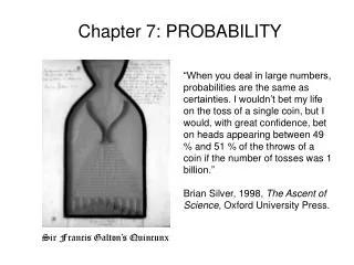
Chapter 7: PROBABILITY “When you deal in large numbers, probabilities are the same as certainties. I wouldn’t bet my life on the toss of a single coin, but I would, with great confidence, bet on heads appearing between 49 % and 51 % of the throws of a coin if the number of tosses was 1 billion.” Brian Silver, 1998, The Ascent of Science, Oxford University Press. Sir Francis Galton’s Quincunx
Histogram Time record Histogram 10 digital values: 1.5, 1.0, 2.5, 4.0, 3.5, 2.0, 2.5, 3.0, 2.5 and 0.5 V resorted in order: 0.5, 1.0, 1.5, 2.0, 2.5, 2.5, 3.0, 3.5, 4.0 V N = 9 occurrences; j = 8 cells; nj = occurrences in j-th cell The histogram is a plot of nj (ordinate) versus magnitude (abscissa).
Proper Choice of Δx The choice of Δx is critical to the interpretation of the histogram. ← made using 3histos.m
Δx Choices Typically, we construct equal-width-interval histograms.
Histogram Construction Rules • To construct equal-width histograms: • Identify the minimum and maximum values of x and its range where xrange = xmax – xmin. • Determine K class intervals (usually use K = 1.15N1/3). • Calculate Δx = xrange / K. • Determine nj (j = 1 to K) in each Δx interval. Note ∑nj = N. • Check that nj > 5 and Δx ≥ ux. • Plot nj versus xmj,where xmj is the midpoint value of each interval.
Frequency Distribution The frequency distribution is a plot of nj /N versus magnitude. It is very similar to the histogram. ← made using hf.m Figure 7.7
Probability Density Function Concept • Consider a signal that varies in time. Figure 7.8 • What is the probability that the signal at a future time will reside between • x and x + Dx?
For x(t): fj /Dx • For n occurrences: Probability Density Function (pdf) • Definition:
In-Class Example • Determine the probability that x is between 1 and 7.
A consequence of this is that PDF pdf Figure 7.14 Probability Distribution Function (PDF) • The probability distribution function (PDF) is related to the integral of the pdf.
When the pdf is ‘normalized’ correctly: Normalization of the pdf Here, >> not normalized So, define pnew(x) = 1/3 p(x) such that
Integrating the pdf expressions give In-Class Example • Determine the expressions for the PDF curve, knowing that of the pdf curve.
The Normal pdf and PDF Figure 8.4