Production, Costs, and Supply

1. Production, Costs, and Supply Principles of Microeconomics Professor Dalton ECON 202 – Fall 2013

2. Production • Production is an activity where resources are altered or changed and there is an increase in the ability of these resources to satisfy wants. • change in physical characteristics • change in location • change in time • change in ownership

3. Production and Cost • Production is a technical relationship between a set of inputs or resources and a set of outputs or goods. QX = f( inputs [land, labor, capital], technology, . . . ) [Legal and social/cultural institutions influence the production function.] • Cost functions are the pecuniary relationships between outputs and the costs of production; Cost = f(QX{inputs, technology} , prices of inputs, . . . ) • Cost functions are determined by input prices and production relationships. It is necessary to understand production functions if you are to interpret cost data.

4. Costs • Costs are incurred as a result of production. These are the costs associated with an activity. When inputs or resources are used to produce one good, the other goods they could have been used to produce are sacrificed. • Costs may be in real or monetary terms; • implicit costs • explicit costs

5. Implicit Costs • Opportunity costs or MC should include all costs associated with an activity. Many of the costs are implicit and difficult to measure. • A production activity may adversely affect a person’s health. This is an implicit cost that is difficult to measure. • Another activity may reduce the time for other activities. It may be possible to make a monetary estimate of the value.

6. Explicit Costs • Explicit costs are those costs where there is an actual expenditure in a market. The costs of labour or interest payments are examples. • Some implicit costs are estimated and used in the decision process. Depreciation is an example.

7. Normal Profit • In neoclassical economics, all costs should be included: • wages represent the cost of labor • Rental rate of capital represents the cost of capital • Rental rate of land represents the cost of land • “normal profit [π]” represents the cost of entrepreneurial activity • normal profit includes reward for risk-bearing

8. Production Function • A production function expresses the relationship between a set of inputs and the output of a good or service. • The relationship is determined by the nature of the good and technology. • A production function is “like” a recipe for cookies; it tells you the quantities of each ingredient, how to combine and cook, and how many cookies you will produce.

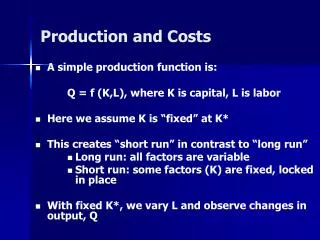
9. QX = f(L, K, R, technology, . . . ) QX = quantity of output L = labor input K = capital input R = natural resources [land] Decisions about alternative ways to produce good X requirethat we have information about how each variable influencesQX. One method used to identify the effects of each variable onoutput is to vary one input at a time. The use of the ceterisparibusconventionallows this analysis. The time period used for analysis also provides a way to determine the effects of various changes of inputs on the output.

10. Technology • The production process [and as result, costs] is divided up into various time periods; • the “very long run” is a period sufficiently long enough that technology used in the production process changes. • In shorter time periods [long run, short run and market periods], technology is a constant.

11. Long Run • The long run is a period that: • is short enough that technology is unchanged. • all other inputs [labor, capital, land, . . . ] are variable, i.e. can be altered. • these inputs may be altered in fixed or variable proportions. This may be important in some production processes. • If inputs are altered, the output changes. • QX = f(L, K, R, . . . ) technology is constant

12. Short Run • The short run is a period: • in which at least one of the inputs has become a constant and at least one of the inputs is a variable. • If capital [K] and land [R] are fixed or constant in the short run, labor [L] is the variable input. Output is changed by altering the labour input. QX = f(L) Technology, K and R are fixed or constant.

13. Market Period • When Alfred Marshall included time into the analysis of production and cost, he included a “market period” in which inputs, technology and consequently outputs could not be varied. • The supply function would be perfectly inelastic in this case.

14. Production of Good X L TPL APL MPL TPL APL = L DTPL MPL = DL 5 29 5.8 4 3 5.3 32 6 34 7 4.87 2 1 4.37 8 35 0 3.89 9 35 Production in the Short Run Consider a production process where K, R and technology arefixed: As L is changed, the outputchanges, QX= f(L) L = labor input TPL = QX = output of good X APL = average product [TP/L] MPL = Marginal product [DTP/ DL] -- 0 0 0 1 4 4 4 5 6 10 2 20 10 3 6.67 5 4 25 6.25 Maximum of APL is at the 3 input oflabor.

15. Production of Good X L TPL APL MPL -- 0 0 0 1 4 4 4 5 6 10 2 20 10 3 6.67 5 4 25 6.25 5 29 5.8 4 3 5.3 32 6 34 7 4.87 2 1 4.37 8 35 0 3.89 9 35 Production in the Short Run Notice that the APL increases as the firstthree units of labor are added to the fixed inputs of K and R. The maximum efficiency of Labor or maximum APL , givenour technology, plant and natural resources is with the third worker. As additional units of labor are addedbeyond the third worker the output per worker [APL ] declines.

16. TPL L 0 0 Output, QX 4 1 35 10 2 30 20 3 25 25 4 20 5 29 15 32 6 10 34 7 5 8 35 9 35 1 2 3 4 5 6 7 8 9 Labor Graphically TPL can be shown: TPL initially increases at an increasingrate; it is convex from below. . . . . TPL . . Maximumoutput . After some point it then increases at a decreasing rate and reaches a maximum level of output, . . . and declines

17. TPL L APL 0 0 0 4 1 4 5 10 2 20 3 6.67 25 4 6.25 10 5 29 5.8 8 5.3 32 6 6 34 7 4.87 4 4.37 8 35 2 3.89 9 35 1 2 3 4 5 6 7 8 9 Labor Given the TP , the APL can calculated: TPL APL = L APL . . . . . . . . . . APL

18. . . . Output, QX TPL Z Z 35 30 25 M 20 H 15 10 5 4 1 2 3 4 5 6 7 8 9 10 Labor 8 6 4 2 1 2 3 4 5 6 7 8 9 Labor . . The APL is theslope of aray fromthe originto theTPL . . Graphically the relationshipbetweenAPLand TPLcan be shown: . 1 unit of L produces 4Q, rise/run = 5 APLis 4/1 = 4 or the slope of line 0H. . 2 units of L produces 10Q, rise/run = 4 . APLis 10/2 = 5 or the slope of line 0M. . 3 units of L produces 20Q, 0 APL . APLis 20/3 = 6.67 or slope of line 0Z. . . . . . As additional units of L are added, AP falls. . . . The maximum AP is where the ray with the greatest slope is tangent to the TP. . APL

19. . . Output, QX 35 30 25 L TPL MPL 20 -- 0 0 4-0 15 1 4 4 6 10 10 2 20 10 3 5 4 4 5 25 1 2 3 4 5 6 7 8 9 10 5 29 4 Labor 3 8 32 6 34 7 2 6 1 8 35 4 0 9 35 2 1 2 3 4 5 6 7 8 9 Labor . . TPL . . MPL was calculated asthe change in TPL given achange in L. . The first unit of labor added4 units of output. . “Between” the 1st and 2cd unitsof labor, Q increases by 6. . . 0 APL . . . . . . . Note: Where MPL = APL, APL is a maximum. . . . . MPL = APL . . . . . . . APL MPL Remember: MP is graphed at “between” units of L.

20. . . Output, QX Z 35 30 25 20 15 10 5 4 1 2 3 4 5 6 7 8 9 10 Labor 8 6 4 2 1 2 3 4 5 6 7 8 9 Labor . . TPL . Useful things to notice: 1. MPL is the slope of TPL. . 2. When TPL increases at an increasing rate, MPL increases. At the inflection point in the TPL , MPL is a maximum. When TPL increases at a decreasing rate,MPL is decreasing. . . . . 3. The APL is a maximum when: a. MPL = APL ,b. the slope of the ray from origin is tangent to TPL . 0 APL . . . . . . . . . . 4. When MPL > APL the APL is increasing. When MPL < APL the APL is decreasing. . . . . . . . . 5. When MPL is 0, theslope of TPL is 0, and TPis a maximum. APL MPL

21. TPL PRODUCTION APL = L LABOUR KAPITAL OUTPUT MP AP 0 5 0 1 5 8 2 5 23 3 5 42 4 5 57 5 5 67 6 5 74 7 5 79 8 5 82 DTPL 9 5 83 MPL = 10 5 82 DL To calculate AP: AP is a maximumwhen L = 4. 8.0 8 11.5 15 Note that MP is 15 between 3rd & 4th units of L, it is 10 between 4th & 5th, so it equals AP = 14.25 at L=4. 19 14.0 15 14.25 10 13.4 7 12.33 5 11.28 3 10.25 To calculate MP: 1 9.22 -1 8.2 MP is a maximum between 2cd and 3rd unit of L.

22. PRODUCTION LABOUR CAPITAL OUTPUT MP AP 0 0 5 0 8.0 8 1 5 8 11.5 15 2 5 23 19 14.0 3 5 42 15 14.25 4 5 57 10 13.4 5 5 67 7 12.33 6 5 74 5 11.28 7 5 79 3 10.25 8 5 82 1 9.22 9 5 83 -1 8.2 10 5 82 As L is added to productionprocess, output per worker [AP]increases. to a maximum “efficiency” [output/input whichoccurs at L = 4. MP increases to a max betweenthe 2cd & 3rd units of L. When MP > AP the output per worker is increasing. Division of Labour and a moreefficient mix of L, K & R causesAP to increase. Output per worker decreases after the 4th worker. “Too many” workers for K, R & tech,MP< AP. Diminishing Marginal Productivity begins with the 4rth unit of L.

23. The price of labour [PL] is $4 per unit and the price of kapital [PK] is $6 per unit. Calculate the cost functions for this production process. PRODUCTION AND COST LABOR CAPITAL OUTPUT AP MP TFC TVC TC AFC AVC ATC 0 5 0 0 -- $30 1 5 8 8 8 $30 2 5 23 11.5 15 $30 3 5 42 14 19 $30 4 5 57 14.25 15 $30 5 5 67 13.4 10 $30 6 5 74 12.33 7 $30 7 5 79 11.28 5 $30 8 5 82 10.25 3 $30 9 5 83 9.22 1 $30 10 5 82 8.2 -1 $30 TFC = PK x K = $6K = 6 x5 = $30, This cost does not change in the short run. TVC = PL x L = $4L, as L changes TVC and Output change. TC = TVC+TFC + =$30 $ 0 $ 4 + =$34 $ 8 + =$38 + =$42 $12 $16 + =$46 $20 + =$50 + =$54 $24 + =$58 $28 + =$62 $32 $36 + =$66 $40 + =$70

24. The price of labor [PL] is $4 per unit and the price of capital [PK] is $6 per unit. Calculate the cost functions for this production process. PRODUCTION AND COST LABOR CAPITAL OUTPUT AP MP TFC TVC TC AFC AVC ATC 0 0 $30 0 5 -- $ 0 $30 1 5 8 8 8 $34 $ 4 $30 2 5 23 11.5 15 $ 8 $38 $30 3 5 42 14 19 $42 $12 $30 4 5 57 14.25 15 $46 $16 $30 5 5 67 13.4 10 $50 $20 $30 6 5 74 12.33 7 $54 $30 $24 7 5 79 11.28 5 $58 $30 $28 8 5 82 10.25 3 $62 $30 $32 9 5 83 9.22 1 $66 $30 $36 10 5 82 8.2 -1 $70 $40 $30 ATC = AVC + AFC = TC¸Q AFC = TFC¸Q = $30¸Q AVC = TVC ¸ Q $4.25 $3.75 $ .50 $1.65 $ .35 $1.30 $1.00 $ .71 $ .29 $.81 $ .28 $ .53 $ .45 $ .30 $.75 $ .32 $.729 $ .41 $.734 $ .38 $ .35 $ .39 $.76 $ .37 $ .36 $ .43 $.79 $ .49 $.86 $ .37

25. PRODUCTION AND COST LABOR CAPITAL OUTPUT AP MP TFC TVC TC AFC AVC ATC 0 0 $30 0 5 -- $ 0 $30 1 5 8 8 8 $34 $4.25 $ 4 $3.75 $ .50 $30 2 5 23 11.5 15 $ 8 $38 $1.65 $ .35 $1.30 $30 3 5 42 14 19 $1.00 $ .71 $ .29 $42 $12 $30 4 5 57 14.25 15 $46 $.81 $ .28 $ .53 $16 $30 5 5 67 13.4 10 $50 $ .45 $ .30 $.75 $20 $30 6 5 74 12.33 7 $ .32 $.729 $54 $ .41 $30 $24 7 5 79 11.28 5 $.734 $ .38 $ .35 $58 $30 $28 8 5 82 10.25 3 $ .39 $62 $.76 $ .37 $30 $32 9 5 83 9.22 1 $66 $30 $ .36 $36 $ .43 $.79 10 5 82 8.2 -1 $ .49 $.86 $70 $ .37 $40 $30 Things to note . . . As AP increases, Since AFC declines, it will “pull”the ATC down as Q increasesbeyond the minimum of the AVC. AVC decreases. When AP is a maximum, AVC is a minimum. AFC declines so long as Q or output increases. {Up to the point where TP becomes negative.}

26. APL APL MPL $ 1 MC x w MC = MPL MPL APL AVC 1 x w AVC = APL AVC The average variable cost [AVC] and marginal cost [MC] are “mirror” imagesof the AP and MP functions. MPL APL APL MPL L L1 L2 L3 L3 The maximum of the AP is consistent with the minimum of the AVC. Q APLx L2

27. MC ATC AVC R J MC will intersect the AVC at theminimum of the AVC [always]. $ ATC* MC will intersect the ATC at the minimum of the ATC. AVC* The vertical distance betweenATC and AVC at any output isthe AFC. At Q** AFC is RJ. Q** Q* Q At Q* output, the AVC is at a minimum AVC* [also max of APL]. At Q** the ATC is at a MINIMUM.

28. The Long Run • The long run is a period of time where: • technology is constant • All inputs are variable • The long run period is a series of short run periods. • For each short run period there is a set of TP, AP, MP, MC, AFC, AVC, ATC, TC, TVC & TFC for each possible scale of plant.

29. MC1 LRMC ATC! MC2 ATC6 ATC2 ATC5 ATC3 ATC* ATC* LRAC LONG RUN COSTS Plant ATC* is the optimal size! $ Cmin At Q* the cost per unit areminimized [the least inputsused]. Q* Q For Plant size 1, the costs are ATC1 and MC1 : For a bigger Plant 2, the unit costs move out and down. It is more cost effective. As bigger plants are built the ATC moves out and down. Eventually, the plant size is “too large,” the ATC moves out but also up! An “envelope curve” is constructed to represent the long run AC [LRAC]. There is a long run marginal cost function.

30. Long Run Average Costs • LRAC is “U-Shaped” • The LRAC initially decreases due to “economies of scale” • economies of scale are due to division of labor. • Eventually, “diseconomies of scale” begin • usually lack of adequate information to manage the production process

31. Calculating LRAC • With a little mathematics, the long run cost functions can be calculated. • It is easier to use equations rather than tables and graphs. • If consumer behavior, production and cost is understood, you can then think about how to achieve your objectives.