Analysis of Variance (ANOVA)
Analysis of Variance (ANOVA). Scott Harris October 2009. Learning outcomes. By the end of this session you should be able to choose between, perform (using SPSS) and interpret the results from: Analysis of Variance (ANOVA), Kruskal-Wallis test,


Analysis of Variance (ANOVA)
E N D
Presentation Transcript
Analysis of Variance (ANOVA) Scott HarrisOctober 2009
Learning outcomes By the end of this session you should be able to choose between, perform (using SPSS) and interpret the results from: • Analysis of Variance (ANOVA), • Kruskal-Wallis test, • Adjusted ANOVA (can also be called Univariate General Linear Model or Multiple linear regression.).
Contents • Reminder of the example dataset. • Comparison of more than 2 independent groups (P/NP) • Test information. • ‘How to’ in SPSS. • Adjusting for additional variables • ‘How to’ in SPSS. • What to do when you add a continuous predictor. • What to do when you add 2 or more categorical predictors. • Interpreting the output.
Example dataset: Information CISR (Clinical Interview Schedule: Revised) data: • Measure of depression – the higher the score the worse the depression. • A CISR value of 12 or greater is used to indicate a clinical case of depression. • 3 groups of patients (each receiving a different form of treatment: GP, CMHN and CMHN problem solving). • Data collected at two time points (baseline and then a follow-up visit 6 months later). • Calculated age at interview from the 2 dates.
Comparing more than two independent groups Analysis of variance (ANOVA) or Kruskal Wallis test
Normally distributed data Analysis of variance (ANOVA)
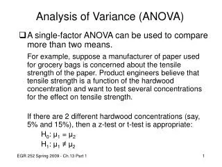
More than 2 groups? When there are more than 2 groups that you wish to compare then t tests are no longer suitable and you should employ Analysis of variance (ANOVA) techniques instead.
Analysis of Variance (ANOVA): Hypotheses The null hypothesis (H0) is that all of the groups are the same. The alternative hypothesis (H1) is that they are not all the same. H1 : Not all the means are the same
SPSS – One-way ANOVA Analyze Compare Means One-Way ANOVA…
SPSS – One-way ANOVA… * One-way ANOVA . ONEWAY B0SCORE BY TMTGR /STATISTICS DESCRIPTIVES /MISSING ANALYSIS /POSTHOC = LSD BONFERRONI ALPHA(.05).
Info: One-way ANOVA in SPSS • From the menus select ‘Analyze’ ‘Compare Means’ ‘One-Way ANOVA…’. • Put the variable that you want to test into the ‘Dependent List:’ box. • Put the categorical variable, that indicates which group the values come from, into the ‘Factor:’ box. • Click the ‘Options’ button and then tick the boxes for ‘Descriptive’. Click ‘Continue’. • Click the ‘Post Hoc…’ button and then tick the boxes for the post hoc tests that you would like. Click ‘Continue’. • Finally click ‘OK’ to produce the test results or ‘Paste’ to add the syntax for this into your syntax file.
SPSS – One-way ANOVA: Output Group summary statistics (descriptives option) 2 sided p value with an alternative hypothesis of non-equality of at least one group. Non significant (P=0.137) hence no significant evidence to suggest differences in the groups.
SPSS – One-way ANOVA: Output… These methods use ‘t tests’ to perform all pair wise comparisons between group means P-value No adjustment for multiple comparisons (LSD option) Adjusted p values for multiple comparisons (Bonferroni option) Mean difference between Groups I and J 95% Confidence interval for the difference between Groups I and J
Non-normally distributed data Kruskal Wallis test
SPSS – Kruskal Wallis test * Kruskal-Wallis test . NPAR TESTS /K-W=M6SCORE BY TMTGR(1 3) /MISSING ANALYSIS. Analyze Nonparametric Tests K Independent Samples…
Info: Kruskal Wallis test in SPSS • From the menus select ‘Analyze’ ‘Nonparametric Tests’ ‘K Independent Samples…’. • Put the variable that you want to test into the ‘Test Variable List:’ box. • Put the categorical variable, that indicates which group the values come from, into the ‘Grouping Variable:’ box. • Click the ‘Define Range…’ box and then enter the numeric codes for the minimum and maximum of the groups that you want to compare. Click ‘Continue’. • Ensure that the ‘Kruskal-Wallis H’ option is ticked in the ‘Test Type’ box. • Finally click ‘OK’ to produce the test results or ‘Paste’ to add the syntax for this into your syntax file.
SPSS – Kruskal Wallis test: Output Observed mean ranks 2 sided p value with an alternative hypothesis of non-equality of groups. Significant (P=0.025) hence significant evidence that at least one of the groups is different. If you want to find out where the differences are then you need to conduct a series of pair-wise Mann Whitney U tests.
Practical Questions From the course webpage download the file HbA1c.sav by clicking the right mouse button on the file name and selecting Save Target As. The dataset is pre-labelled and contains data on Blood sugar reduction for 245 patients divided into 3 groups. • Assuming that the outcome variable is normally distributed: Conduct a suitable statistical test to compare the finishing HbA1c level (HBA1C_2) between all of the 3 groups. What are your conclusions from this test if you don’t worry about multiple testing? What about if you do, using a Bonferroni correction? • Assuming that the outcome variable is NOTnormally distributed: Conduct a suitable statistical test to compare the finishing HbA1c level (HBA1C_2) between all of the 3 groups. What are your conclusions from this test?
Practical Solutions • The ANOVA table shows that at least one of the groups is significantly different from the others (p=0.010).
Practical Solutions Looking at the individual LSD and Bonferroni corrected pair-wise comparisons it can be seen that there is only one contrast that shows a significant difference at the 5% level and that is Active A vs. Placebo, with the Placebo levels higher.
Practical Solutions • For the non-parametric test, again, there is only a p value to report from the test (although the group medians could be reported from elsewhere, the pair-wise comparisons need to be done as separate Mann-Whitney U tests as shown in Analysing Continuous data and CI’s for these differences could be calculated from CIA). The Kruskal-Wallis test shows that at least one of the groups is significantly different from the others (p=0.013)
Comparing groups and adjusting for other variables Adjusted ANOVA
Adjusted ANOVA Sometimes you wish to look at a relationship that is more complicated than one continuous outcome with one categorical group ‘predictor’. Adjusted ANOVA allows for the addition of other covariates (predictor variables). These can be either categorical, continuous or a combination of both. The next command in SPSS is one of the most powerful. SPSS calls it a Univariate General Linear Model (GLM). It can replicate one-way ANOVA and Linear regression. It is also equivalent to multiple regression but with a bit more flexibility.
Example 1 Replicating the one-way ANOVA
SPSS – Adjusted ANOVA Outcome variable Categorical predictor variables Continuous predictor variables Analyze General Linear Model Univariate…
SPSS – Adjusted ANOVA… Can produce pair-wise comparisons for multiple categorical variables The same additional options can be set as for the one-way ANOVA, with post hoc pair-wise comparisons…
SPSS – Adjusted ANOVA… and simple descriptive statistics available.
Info: Adjusted ANOVA in SPSS(no continuous covariates) • From the menus select ‘Analyze’ ‘General Linear Model’ ‘Univariate…’. • Put the variable that you want to test into the ‘Dependent Variable:’ box. • Put any categorical variables, that indicate which group the values come from or some other category, into the ‘Fixed Factor(s):’ box. • Click the ‘Options’ button and then tick the boxes for ‘Descriptive statistics’. Click ‘Continue’. • Click the ‘Post Hoc…’ button and then move over the categorical variable(s) that you would like the pairwise comparisons for. Then tick the boxes for the post hoc tests that you would like. Click ‘Continue’. • Finally click ‘OK’ to produce the test results or ‘Paste’ to add the syntax for this into your syntax file.
SPSS – Adjusted ANOVA: Output This is the same p value as from the one-way ANOVA and it is interpreted in the same way. Notice how the row uses the variable name (important for later).
SPSS – Adjusted ANOVA: Output… The same post-hoc pair-wise results as before:
Example 2 Adjusting for continuous and categorical covariates
SPSS – Adjusted ANOVA Outcome variable Categorical predictor variables (2 categorical variables here) Continuous predictor variables (1 continuous variable here) Analyze General Linear Model Univariate…
SPSS – Adjusted ANOVA… As soon as we include a continuous covariate, the Post Hoc option is no longer available and we need to use the ‘Contrasts…’ option which isn’t quite as powerful.
SPSS – Adjusted ANOVA… Select the Category that you want the contrast for and then you can select the type of contrast and the reference level. ‘Simple’ is the standard contrast (simple differences between levels) and the reference category is the level that all other levels of the categorical variable are compared against.
Info: Adjusted ANOVA in SPSS(inc. continuous covariates) • From the menus select ‘Analyze’ ‘General Linear Model’ ‘Univariate…’. • Put the variable that you want to test into the ‘Dependent Variable:’ box. • Put any categorical variables, that indicate which group the values come from or some other category, into the ‘Fixed Factor(s):’ box. • Put any continuous variables into the ‘Covariate(s):’ box. • Click the ‘Contrasts…’ button and set up any contrasts that you want for any categorical variables. You need to select the variable, then choose the type of contrast (generally you use ‘Simple’). Next you need to select the reference level. This can be either first or last and it will dictate the level of the category variable that all other levels will be compared against (first will compare all other levels against the first: 2nd -1st, 3rd-1st etc.), then click ‘Change’. When you are finished click ‘Continue’. • Click the ‘Options’ button and then tick the boxes for ‘Descriptive statistics’. Click ‘Continue’. • Finally click ‘OK’ to produce the test results or ‘Paste’ to add the syntax for this into your syntax file.
SPSS – Adjusted ANOVA… If you have more than 1 variable in the ‘Fixed Factor(s)’ box then you need to go into the ‘Model..’ options.
SPSS – Adjusted ANOVA… The default model is ‘Full factorial’. This will include all possible interactions between factors. Generally we want to consider only main effects (at least at the start). To do this select ‘Custom’ and then set ‘Type:’ to ‘Main effects’ and move all ‘Factors & Covariates’ into the ‘Model:’ box.
Info: Adjusted ANOVA in SPSS(2+ categorical covariates) • From the menus select ‘Analyze’ ‘General Linear Model’ ‘Univariate…’. • Put the variable that you want to test into the ‘Dependent Variable:’ box. • Put the 2 or more categorical variables, that indicate which group the values come from or some other category, into the ‘Fixed Factor(s):’ box. • Click the ‘Model…’ button and then select ‘Custom…’. Change the ‘Type:’ type to ‘Main effects’ and then move all ‘Factors & Covariates’ into the Model:’ box. • Put any continuous variables into the ‘Covariate(s):’ box. • Set up either the ‘Post Hoc…’ or ‘Contrasts…’ options depending on whether there are any continuous covariates or not (see previous information slides). • Click the ‘Options’ button and then tick the boxes for ‘Descriptive statistics’. Click ‘Continue’. • Finally click ‘OK’ to produce the test results or ‘Paste’ to add the syntax for this into your syntax file.
SPSS – Adjusted ANOVA: Output Descriptive statistics separated by all combinations of the factor variables. This is now the p-value for the effect of TMTGR having adjusted for SEX and AgeInt. So having taken into account variability due to SEX and AgeInt there is no statistically significant difference between the treatment groups (p=0.121). Similar statements can be made regarding the other variables in the model, i.e. having adjusted for TMTGR and AgeInt there is no statistically significant difference between the 2 sexes (p=0.261).
SPSS – Adjusted ANOVA: Output… The Contrast results (interpretation is the same as the previous slide): The TMTGR variable had 3 levels here: 1 – GP 2 – CMHN 3 – CMHN PS By selecting the first level of the factor as the reference category the contrast will produce: CMHN – GP (2-1) CMHN PS – GP (3-1) 95% CI for the difference between CMHN PS and GP P-value for CMHN PS - GP Difference between CMHN PS and GP
Practical Questions • Using an Adjusted ANOVA with the finial HbA1c level (HBA1C_2) as the outcome: • Replicate the model from question 1. • Add the baseline level of HbA1c (HBA1C_1) in as a covariate. How does this affect the results? • Add Gender to the model from part (ii). Look at just the main effects of the variables rather than any interactions. Does this change your results? Do you think Gender should be in the model?
Practical Solutions 3) i. By adding HBA1C_2 as the dependent variable and GROUP as a Fixed factor we can replicate the one-way ANOVA
Practical Solutions The same multiple comparisons:
Practical Solutions 3) ii. By adding HBA1C_1 to the model GROUP has become more significant. We are explaining an additional amount of variability, hence increasing the precision.
Practical Solutions We need to use the contrasts option when a continuous covariate is added to the model. To see the remaining contrast we need to re-run with a different reference category.
Practical Solutions 3) iii. Adding in another categorical covariate means we need to go into the model options or we will get interaction terms fitted as default.
Practical Solutions The size of the effects alters slightly but the conclusion remains the same. Although Gender is not statistically significant it may still be important in the model. We can include terms if they are significant in our sample, they are key variables that have shown to be important in the literature or we want to test them for differences.