Standard Deviation for Grouped D ata
Standard Deviation for Grouped D ata. 2.4 - 2.5 . Finding the Standard Deviation for Grouped Data. The procedure for finding the variance and standard deviation for grouped data is similar to that for finding the mean for grouped data, and it uses the midpoints of each class.

Standard Deviation for Grouped D ata
E N D
Presentation Transcript
Standard Deviation for Grouped Data 2.4 - 2.5
Finding the Standard Deviation for Grouped Data • The procedure for finding the variance and standard deviation for grouped data is similar to that for finding the mean for grouped data, and it uses the midpoints of each class.
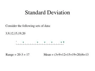
Example • Find the variance and the standard deviation for the frequency distribution of the data. The data represent the number of miles that 20 runners ran during one week.
Make the table shown, and find the midpoint for each class Multiply the frequency by the midpoint for each class, and place the products in the 4th column Multiply the frequency by the square of the midpoint, he products and place the 5th column. Find the sums of the 2nd, 4th and 5th column.
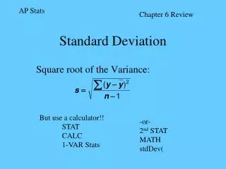
Apply formula • =20(45,002)-4902/20(20-1) • =900,040-240,100/20(19) • =659,940/380 • =1736.68 • Take the square root to get the standard deviation • S= √ 1736.68 = 41.67 • Be sure to use the number found in the sum of the 2nd column for n. Do not use the number of classes.
Range Rule of Thumb • The range can be used to approximate the standard deviation. The approximation is called the range rule of thumb. • S ≈ range/4 • Example: The data set 5, 8, 8, 9, 10, 12, and 13, has a standard deviation o f 2.7 and the range is 13-5= 8 The range rule of thumb is s≈ 2. • In this example the range rule of thumb underestimates the standard deviation but it is in the ballpark.
Range Rule of Thumb • The range rule of thumb can be used to estimate the largest and smallest data values of a data set. The smallest value will be approximately 2 standard deviations below the mean, and the largest data value will be approximately 2 standard deviations above the mean of the data set. • Example the mean from the data set 5, 8, 8, 9, 10, 12, and 13, is 9.3 hence, • Smallest data value = X - 2s = 9.3 - 2(2.8) = 3.7 • Largest data value = X + 2s = 9.3 + 2(2.8) = 14.9 • Now look back at the original data set. The Smallest was 5 and the largest was 13. Again these are considered rough estimates. Better approximations can be obtained by using Chebyshev’s theorem and the empirical rule.
Chebychev’s Theorem • The portion of values from any data set lying within z standard deviations (z>1) of the mean is at least 1 – 1/z2. • Z = 2: In any data set, at least 1 – 1/22 = ¾, or 75%, of the data lie within 2 standard deviations of the mean. • Z=3: In any data set, at least 1 – 1/32 = 8/9, or 88.9%, of the data lie within 3 standard deviations of the mean. • Applies to any distribution regardless of it’s shape.
Chebychev’s Theorem Example The age distributions for Alaska and Florida are shown in the histograms. Decide which is which. Apply Chebychev’s Theorem to the data for Florida.
Practice • The mean price of houses in a certain neighborhood is $50,000, and the standard deviation is $10,000. Find the price range for which at least 75% of the houses will sell.
Chebychev’s Theorem • Chebyshev’s theorem can be used to find the minimum percentage of data values that will fall between any two given values. • Example: A survey of local companies found that the mean amount of travel allowances for executives was $0.25 per mile. The standard deviation was $0.02. Using Chebychev’s theorem, find the minimum percentage of the data values that will fall between $0.20 and $0.30.
Empirical Rule • Applies only to bell shaped (NORMAL) distributions • Approximately 68% of the data values will fall within 1 standard deviation of the mean. • Approximately 95% of the data values will fall within 2 standard deviation of the mean. • Approximately 99.7% of the data values will fall within 3 standard deviation of the mean. Data values that lie more than 2 standard deviations from the mean are considered unusual. Data values that lie more than three standard deviations from the mean are very unusual.
Empirical Rule ( or 68-95-99.7 Rule) • Many real-life data sets have distributions that are approximately symmetric and bell shaped. 68% of the data lie within 1 standard deviation 95% of the data lie within 2 standard deviations 99.7% of the data lie within 3 standard deviations
Using the Empirical Rule • In a survey conducted by the National Center for Health Statistics, the sample mean height of women in the U.S. (ages 20-29) was 64 inches with a sample standard deviation of 2.75 inches. Estimate the percent of women whose heights are between 64 inches and 69.5 inches. • We know 64 is the mean to calculate how much 2 standard deviations from the mean is we take the MEAN + 2(STANDARD DEVIATIONS)= or 64+2(2.75)=69.5
Using the Empirical Rule • Because the distribution is bell shaped, you can use the Empirical Rule. • Because the 69.5 is 2 standard deviations above the mean height, the percent of the heights between 64 inches and 69.5 inches is 34% + 13.6 % or 47.6% • So 47.6% of women are between 64 inches and 69.5 inches.