Limits and Their Properties
1. Limits and Their Properties. 1.4. Continuity and One-Sided Limits. Continuity at a Point and on an Open Interval. Continuity at a Point and on an Open Interval.


Limits and Their Properties
E N D
Presentation Transcript
1 Limits and Their Properties
1.4 Continuity and One-Sided Limits
Continuity at a Point and on an Open Interval
Continuity at a Point and on an Open Interval Three values of x at which the graph of f is not continuous. At all other points in the interval (a, b), the graph of f is uninterrupted and continuous.
Continuity at a Point and on an Open Interval Consider an open interval I that contains a real number c. If a function f is defined on I (except possibly at c), and f is not continuous at c, then f is said to have a discontinuity at c. Discontinuities fall into two categories: removable and nonremovable. A discontinuity at c is called removable if f can be made continuous by appropriately defining (or redefining f(c)).
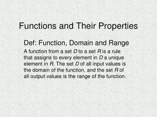
Figure 1.26 Continuity at a Point and on an Open Interval For instance, the functions shown in Figures 1.26(a) and (c) have removable discontinuities at c and the function shown in Figure 1.26(b) has a nonremovable discontinuity at c.
Example 1 – Continuity of a Function Discuss the continuity of each function.
Example 1(a) – Solution The domain of f is all nonzero real numbers. From Theorem 1.3, you can conclude that f is continuous at every x-value in its domain. At x =0, f has Non-Removable Discontinuity. In other words, there is no way to define f(0) so as to make the function continuous at x = 0.
Example 1(b) – Solution cont’d The domain of g is all real numbers except x = 1. From Theorem 1.3, you can conclude that g is continuous at every x-value in its domain. At x = 1, the function has Removable discontinuity. If g(1) is defined as 2, the “newly defined” function is continuous for all real numbers.
Example 1(c) – Solution cont’d The domain of h is all real numbers. The function h is continuous on and , and, because , h is continuous on the entire real line.
Example 1(d) – Solution cont’d The domain of y is all real numbers. From Theorem 1.6, you can conclude that the function is continuous on its entire domain, .
One-Sided Limits and Continuity on a Closed Interval To understand continuity on a closed interval, you first need to look at a different type of limit called a one-sided limit. For example, the limit from the right (or right-hand limit) means that x approaches c from values greater than c. This limit is denoted as
One-Sided Limits and Continuity on a Closed Interval Similarly, the limit from the left (or left-hand limit) means that x approaches c from values less than c. This limit is denoted as
Example 2 – A One-Sided Limit Find the limit of f(x) = as x approaches –2 from the right. Solution: The limit as x approaches –2 From the right is
One-Sided Limits and Continuity on a Closed Interval One-sided limits can be used to investigate the behavior of step functions. One common type of step function is the greatest integer function , defined by For instance, and
Example 4 – Continuity on a Closed Interval Discuss the continuity of f(x)= Solution: The domain of f is the closed interval [–1, 1]. At all points in the open interval (–1, 1), the continuity of f follows from Theorems 1.4 and 1.5.
Example 4 – Solution cont’d Moreover, because and you can conclude that f is continuous on the closed interval [–1, 1]
Example 7 – Testing for Continuity Describe the interval(s) on which each function is continuous.
Example 7(a) – Solution The tangent function f(x) = tan x is undefined at At all other points it is continuous.
Example 7(a) – Solution cont’d So, f(x) = tan x is continuous on the open intervals
Example 7(b) – Solution cont’d Because y = 1/x is continuous except at x = 0 and the sine function is continuous for all real values of x, it follows that y = sin (1/x) is continuous at all real values except x = 0. At x = 0, the limit of g(x) does not exist. So, g is continuous on the intervals
Example 7(c) – Solution cont’d This function is similar to the function in part (b) except that the oscillations are damped by the factor x. Using the Squeeze Theorem, you obtain and you can conclude that So, h is continuous on the entire real line.
The Intermediate Value Theorem The Intermediate Value Theorem tells you that at least one number c exists, but it does not provide a method for finding c. Such theorems are called existence theorems. The Intermediate Value Theorem states that for a continuous function f, if x takes on all values between a and b, f(x)must take on all values between f(a) and f(b).
The Intermediate Value Theorem Suppose that a girl is 5 feet tall on her thirteenth birthday and 5 feet 7 inches tall on her fourteenth birthday. Then, for any height h between 5 feet and 5 feet 7 inches, there must have been a time t when her height was exactly h. This seems reasonable because human growth is continuous and a person’s height does not abruptly change from one value to another.
The Intermediate Value Theorem The Intermediate Value Theorem guarantees the existence of at least one number c in the closed interval [a, b] . There may, of course, be more than one number c such that f(c) = k.
The Intermediate Value Theorem A function that is not continuous does not necessarily exhibit the intermediate value property. For example, the graph of the function shown in Figure 1.36 jumps over the horizontal line given by y =k, and for this function there is no value of c in [a, b] such that f(c) = k. Figure 1.36
The Intermediate Value Theorem The Intermediate Value Theorem often can be used to locate the zeros of a function that is continuous on a closed interval. Specifically, if f is continuous on [a, b] and f(a) and f(b) differ in sign, the Intermediate Value Theorem guarantees the existence of at least one zero of f in the closed interval [a, b] .
Example 8 – An Application of the Intermediate Value Theorem Use the Intermediate Value Theorem to show that the polynomial function has a zero in the interval [0, 1]. Solution: Note that f is continuous on the closed interval [0, 1]. Because it follows that f(0) < 0 and f(1) > 0.
Example 8 – Solution cont’d You can therefore apply the Intermediate Value Theorem to conclude that there must be some c in [0, 1] such that